(Adding class notes (Converted from LaTeX with latex2wiki)) |
|||
| (23 intermediate revisions by 9 users not shown) | |||
| Line 1: | Line 1: | ||
| − | = | + | <center><font size= 4> |
| + | '''[[ECE662]]: Statistical Pattern Recognition and Decision Making Processes''' | ||
| + | </font size> | ||
| + | Spring 2008, [[user:mboutin|Prof. Boutin]] | ||
| − | + | [[Slectures|Slecture]] | |
| + | <font size= 3> Collectively created by the students in [[ECE662:BoutinSpring08_OldKiwi|the class]]</font size> | ||
| + | </center> | ||
| + | ---- | ||
| + | =Lecture 26 Lecture notes= | ||
| + | Jump to: [[ECE662_Pattern_Recognition_Decision_Making_Processes_Spring2008_sLecture_collective|Outline]]| | ||
| + | [[Lecture 1 - Introduction_OldKiwi|1]]| | ||
| + | [[Lecture 2 - Decision Hypersurfaces_OldKiwi|2]]| | ||
| + | [[Lecture 3 - Bayes classification_OldKiwi|3]]| | ||
| + | [[Lecture 4 - Bayes Classification_OldKiwi|4]]| | ||
| + | [[Lecture 5 - Discriminant Functions_OldKiwi|5]]| | ||
| + | [[Lecture 6 - Discriminant Functions_OldKiwi|6]]| | ||
| + | [[Lecture 7 - MLE and BPE_OldKiwi|7]]| | ||
| + | [[Lecture 8 - MLE, BPE and Linear Discriminant Functions_OldKiwi|8]]| | ||
| + | [[Lecture 9 - Linear Discriminant Functions_OldKiwi|9]]| | ||
| + | [[Lecture 10 - Batch Perceptron and Fisher Linear Discriminant_OldKiwi|10]]| | ||
| + | [[Lecture 11 - Fischer's Linear Discriminant again_OldKiwi|11]]| | ||
| + | [[Lecture 12 - Support Vector Machine and Quadratic Optimization Problem_OldKiwi|12]]| | ||
| + | [[Lecture 13 - Kernel function for SVMs and ANNs introduction_OldKiwi|13]]| | ||
| + | [[Lecture 14 - ANNs, Non-parametric Density Estimation (Parzen Window)_OldKiwi|14]]| | ||
| + | [[Lecture 15 - Parzen Window Method_OldKiwi|15]]| | ||
| + | [[Lecture 16 - Parzen Window Method and K-nearest Neighbor Density Estimate_OldKiwi|16]]| | ||
| + | [[Lecture 17 - Nearest Neighbors Clarification Rule and Metrics_OldKiwi|17]]| | ||
| + | [[Lecture 18 - Nearest Neighbors Clarification Rule and Metrics(Continued)_OldKiwi|18]]| | ||
| + | [[Lecture 19 - Nearest Neighbor Error Rates_OldKiwi|19]]| | ||
| + | [[Lecture 20 - Density Estimation using Series Expansion and Decision Trees_OldKiwi|20]]| | ||
| + | [[Lecture 21 - Decision Trees(Continued)_OldKiwi|21]]| | ||
| + | [[Lecture 22 - Decision Trees and Clustering_OldKiwi|22]]| | ||
| + | [[Lecture 23 - Spanning Trees_OldKiwi|23]]| | ||
| + | [[Lecture 24 - Clustering and Hierarchical Clustering_OldKiwi|24]]| | ||
| + | [[Lecture 25 - Clustering Algorithms_OldKiwi|25]]| | ||
| + | [[Lecture 26 - Statistical Clustering Methods_OldKiwi|26]]| | ||
| + | [[Lecture 27 - Clustering by finding valleys of densities_OldKiwi|27]]| | ||
| + | [[Lecture 28 - Final lecture_OldKiwi|28]] | ||
| + | ---- | ||
| + | ---- | ||
| − | = | + | =Assignment Update= |
| − | + | *There will not be a final project homework assignment, instead a peer review of the last homework will take place see [[Homework 3_OldKiwi]] for details. | |
| − | + | ||
| − | *There will not be a final homework assignment | + | |
| − | + | ||
| − | + | ||
| − | + | ||
| − | + | ||
| − | + | ||
| − | + | ||
| − | + | ||
| − | + | ||
| − | + | ||
| − | + | ||
| − | + | ||
| − | + | ||
| − | + | ||
| − | + | ||
| − | + | ||
| − | + | ||
| − | + | ||
| − | + | ||
| − | + | ||
| − | + | ||
| − | + | ||
=Clustering= | =Clustering= | ||
| Line 42: | Line 57: | ||
==Minimizing== | ==Minimizing== | ||
| − | <center><math> J=\sum_{j=1}\sum_{x_{i}\in S_{j}}||x_{i}-\mu_{j}||^{2}</math></center> | + | <center><math> J=\sum_{j=1}^c\sum_{x_{i}\in S_{j}}||x_{i}-\mu_{j}||^{2}</math></center> |
<center><math> =\sum_{j=1}^c\frac{1}{|S_{j}|}\sum_{x_{i},x_{k}\in S_{j}}||x_{i}-x_{k}||^{2}is</math></center> | <center><math> =\sum_{j=1}^c\frac{1}{|S_{j}|}\sum_{x_{i},x_{k}\in S_{j}}||x_{i}-x_{k}||^{2}is</math></center> | ||
same as minimizing trace of the within class variation matrix, | same as minimizing trace of the within class variation matrix, | ||
<center><math>J_{within}=\sum_{j=1}^c\sum_{x_{i}\in S_{j}}(x_{i}-\mu_{j})^{T}(x_{i}-x_{j})=\sum_{j=1}^c\sum_{x_{i}\in S_{j}}tr((x_{i}-\mu_{j})(x_{i}-x_{j})^{T})</math></center> | <center><math>J_{within}=\sum_{j=1}^c\sum_{x_{i}\in S_{j}}(x_{i}-\mu_{j})^{T}(x_{i}-x_{j})=\sum_{j=1}^c\sum_{x_{i}\in S_{j}}tr((x_{i}-\mu_{j})(x_{i}-x_{j})^{T})</math></center> | ||
| − | which is the same as maximizing the between-cluster variance<center><math> S_{Total}=S_{W}+S_{B}</math></center> <center><math> tr(S_{w})=tr(S_{Total})-tr(S_{B})</math></center> Since the total variance, <math>S_{Total}</math>, does not change, maximizing the between-class variance is equivalent to minimizing the within-class variance. | + | which is the same as maximizing the between-cluster variance<center><math> S_{Total}=S_{W}+S_{B}</math></center> <center><math> tr(S_{w})=tr(S_{Total})-tr(S_{B})</math></center> |
| − | + | ||
| + | |||
| + | So, <math> \min S_w = \min ( tr(S_{total}) - tr(S_B) ) = tr(S_{total})+\min(-tr(S_B)) </math> | ||
| + | |||
| + | Therefore, <math> \min tr(S_w) </math> is attained at <math> tr(S_B) </math> | ||
| + | |||
| + | |||
| + | |||
| + | Since the total variance, <math>S_{Total}</math>, does not change, maximizing the between-class variance is equivalent to minimizing the within-class variance. | ||
| + | |||
| + | == Comment about decision surfaces == | ||
| + | This sub-section is a stub. You can help by adding what Mimi said about this topic. | ||
=Statistical Clustering Methods= | =Statistical Clustering Methods= | ||
| Line 53: | Line 79: | ||
Clustering by mixture decomposition works best with Gaussians. What | Clustering by mixture decomposition works best with Gaussians. What | ||
are examples of gaussians? Circles, ellipses. However, if you have | are examples of gaussians? Circles, ellipses. However, if you have | ||
| − | banana-like data, that won't work so well. | + | banana-like data, that won't work so well. |
| − | to earlier discussion of this concept?] | + | |
| + | [[Article idea, with links to earlier discussion of this concept?_OldKiwi]] | ||
If you are in higher dimensions, do not even think of using statistical | If you are in higher dimensions, do not even think of using statistical | ||
clustering methods! There is simply too much space through which the | clustering methods! There is simply too much space through which the | ||
data is spread, so they won't be lumped together very closely. | data is spread, so they won't be lumped together very closely. | ||
| − | |||
*Assume each pattern <math>x_{i}\in D</math> was drawn from a mixture <math>c</math> underlying populations. (<math>c</math> is the number of classes) | *Assume each pattern <math>x_{i}\in D</math> was drawn from a mixture <math>c</math> underlying populations. (<math>c</math> is the number of classes) | ||
| Line 70: | Line 96: | ||
Then the separation between the clusters is given by the separation | Then the separation between the clusters is given by the separation | ||
surface between the classes (which is defined as ...)\\ | surface between the classes (which is defined as ...)\\ | ||
| − | |||
| + | [[Image:Lec26_Fig_valley_mean_OldKiwi.JPG]] (Fig.1) | ||
| + | |||
| + | Note that this process gives a set of pair-wise seperations between classes/categories. To generalize to a future data point, need to collect the decisions on all pair-wise seperations and then use the rule of majority vote to decide which class the point should be assigned to. | ||
==Example: Model the data as a Gaussian Mixture== | ==Example: Model the data as a Gaussian Mixture== | ||
| Line 92: | Line 120: | ||
If <math>\Sigma_{1},\Sigma_{2},\ldots,\Sigma_{c}</math> are not all equal, this | If <math>\Sigma_{1},\Sigma_{2},\ldots,\Sigma_{c}</math> are not all equal, this | ||
is the same as minimizing<center><math> | is the same as minimizing<center><math> | ||
| − | \prod_{i=1}^|S_{W}^{(i)}|</math></center> | + | \prod_{i=1}^c|S_{W}^{(i)}|</math></center> |
| + | == Professor Bouman's "Cluster" Software == | ||
| + | The "CLUSTER" software, developed by Purdue University's own Professor Charles Bouman, can be found, along with all supporting documentation, here: [http://cobweb.ecn.purdue.edu/~bouman/software/cluster/ Cluster Homepage]. The algorithm takes an iterative bottom-up (or agglomerative) approach to clustering. Different from many clustering algorithms, this one uses a so-called "Rissanen criterion" or "minimum description length" ([[MDL_OldKiwi]]) as the best fit criterion. In short, [[MDL_OldKiwi]] favors density estimates with parameters that may be encoded (along with the data) with very few bits. i.e. The simpler it is to represent both the density parameters and data in some binary form, the better the estimate is considered. | ||
| + | Note: there is a typo in the manual that comes with "CLUSTER." In the overview figure, two of the blocks have been exchanged. The figure below hopefully corrects this typo. | ||
| − | + | Below is the block diagram from the software manual (with misplaced blocks corrected) describing the function of the software. | |
| − | + | [[Image:BoumanClusterBlockDiagram_OldKiwi.jpg]] (Fig.2) | |
| − | + | ||
| − | + | ||
| − | + | ||
| − | + | ||
| − | + | ||
| − | + | ||
| − | + | ||
| − | + | ||
| − | + | ||
| − | + | ||
| − | + | ||
| − | + | ||
| − | + | ||
| − | + | ||
| − | + | ||
| − | + | ||
| − | + | ||
| − | + | ||
| − | + | ||
| − | + | ||
| − | + | ||
| − | + | ||
=Clustering by finding valleys of densities= | =Clustering by finding valleys of densities= | ||
| Line 128: | Line 137: | ||
in 2D | in 2D | ||
| − | + | [[Image:Lec26_Fig_valley_OldKiwi.JPG]] (Fig.3) | |
Advantages | Advantages | ||
| − | |||
*no presumptions about the shape of the data | *no presumptions about the shape of the data | ||
*no presumptions about the number of clusters | *no presumptions about the number of clusters | ||
| − | |||
| − | + | ==Approach 1: "bump hunting" == | |
| + | Reference: CLIQUE98 Agrawal ''et al.'' | ||
| − | *Approximate the density fct p(x), (Parzen window) | + | *Approximate the density fct p(x), (Using Parzen window) |
| + | *Approximate the density fct p(x), (Using K-Nearest Neighbor) | ||
| + | == References == | ||
| + | * CLIQUE98 Agrawal ''et al.'' | ||
| − | + | [[Category:ECE662]] | |
| − | + | [[Category:decision theory]] | |
| − | + | [[Category:Lecture Notes]] | |
| − | + | [[Category:pattern recognition]] | |
| − | [[ | + | [[Category:slecture]] |
Latest revision as of 11:24, 10 June 2013
ECE662: Statistical Pattern Recognition and Decision Making Processes
Spring 2008, Prof. Boutin
Collectively created by the students in the class
Contents
Lecture 26 Lecture notes
Jump to: Outline| 1| 2| 3| 4| 5| 6| 7| 8| 9| 10| 11| 12| 13| 14| 15| 16| 17| 18| 19| 20| 21| 22| 23| 24| 25| 26| 27| 28
Assignment Update
- There will not be a final project homework assignment, instead a peer review of the last homework will take place see Homework 3_OldKiwi for details.
Clustering
- There are no best criterion for obtaining a partition of $ \mathbb{D} $
- Each criterion imposes a certain structure on the data.
- If the data conforms to this structure, the true clusters can be discovered.
- There are very few criteria which can be both handled mathematically and understood intuitively. If you can develope a useful intuitive criterion and describe and optimize it mathematically, you can make big contributions to this field.
- Some criteria can be written in different ways, for example minimizing the square error, as in the following section.
Minimizing
same as minimizing trace of the within class variation matrix,
So, $ \min S_w = \min ( tr(S_{total}) - tr(S_B) ) = tr(S_{total})+\min(-tr(S_B)) $
Therefore, $ \min tr(S_w) $ is attained at $ tr(S_B) $
Since the total variance, $ S_{Total} $, does not change, maximizing the between-class variance is equivalent to minimizing the within-class variance.
Comment about decision surfaces
This sub-section is a stub. You can help by adding what Mimi said about this topic.
Statistical Clustering Methods
Clustering by mixture decomposition works best with Gaussians. What are examples of gaussians? Circles, ellipses. However, if you have banana-like data, that won't work so well.
Article idea, with links to earlier discussion of this concept?_OldKiwi
If you are in higher dimensions, do not even think of using statistical clustering methods! There is simply too much space through which the data is spread, so they won't be lumped together very closely.
- Assume each pattern $ x_{i}\in D $ was drawn from a mixture $ c $ underlying populations. ($ c $ is the number of classes)
- Assume the form for each population is known
- Define the mixture density
- Use pattern's $ x_{i}'s $ to estimate $ \theta $ and the priors $ P(\omega_{i}) $
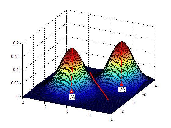
Then the separation between the clusters is given by the separation surface between the classes (which is defined as ...)\\
Note that this process gives a set of pair-wise seperations between classes/categories. To generalize to a future data point, need to collect the decisions on all pair-wise seperations and then use the rule of majority vote to decide which class the point should be assigned to.
Example: Model the data as a Gaussian Mixture
$ p(x|\mu_{i},\ldots,\mu_)=\sum_{i=1}^cP(\omega_{i})\frac{e^{(x_{1}-\mu_{1})^{T}\Sigma_{1}^{-1}(x_{1}-\mu_{1})}}{2\pi|\Sigma_{i}|^{n/2}} $
Note: the Maximum Likelihood approach to estimating $ \theta $is the same as minimizing the cost function $ J $ of the between-class scatter matrices.
Sub-example
If $ \Sigma_{1}=\Sigma_{2}=\ldots=\Sigma_{c} $, then this is the same as minimizing $ |S_{w}| $
Sub-example 2
If $ \Sigma_{1},\Sigma_{2},\ldots,\Sigma_{c} $ are not all equal, this
is the same as minimizingProfessor Bouman's "Cluster" Software
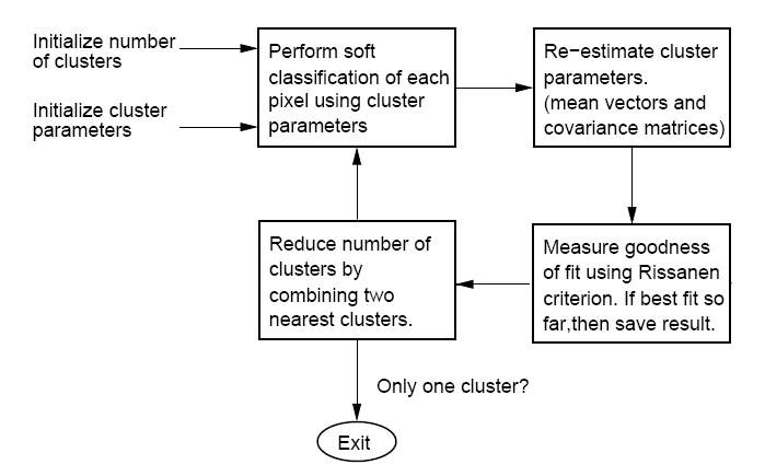
The "CLUSTER" software, developed by Purdue University's own Professor Charles Bouman, can be found, along with all supporting documentation, here: Cluster Homepage. The algorithm takes an iterative bottom-up (or agglomerative) approach to clustering. Different from many clustering algorithms, this one uses a so-called "Rissanen criterion" or "minimum description length" (MDL_OldKiwi) as the best fit criterion. In short, MDL_OldKiwi favors density estimates with parameters that may be encoded (along with the data) with very few bits. i.e. The simpler it is to represent both the density parameters and data in some binary form, the better the estimate is considered.
Note: there is a typo in the manual that comes with "CLUSTER." In the overview figure, two of the blocks have been exchanged. The figure below hopefully corrects this typo.
Below is the block diagram from the software manual (with misplaced blocks corrected) describing the function of the software.
 (Fig.2)
Clustering by finding valleys of densities
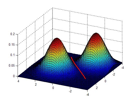
Idea: Cluster boundaries correspond to local minima of density fct (=valleys)
in 2D
Advantages
- no presumptions about the shape of the data
- no presumptions about the number of clusters
Approach 1: "bump hunting"
Reference: CLIQUE98 Agrawal et al.
- Approximate the density fct p(x), (Using Parzen window)
- Approximate the density fct p(x), (Using K-Nearest Neighbor)
References
- CLIQUE98 Agrawal et al.


