ECE662: Statistical Pattern Recognition and Decision Making Processes

Spring 2008, Prof. Boutin

Collectively created by the students in the class

Lecture 16 Lecture notes

Jump to: Outline| 1| 2| 3| 4| 5| 6| 7| 8| 9| 10| 11| 12| 13| 14| 15| 16| 17| 18| 19| 20| 21| 22| 23| 24| 25| 26| 27| 28

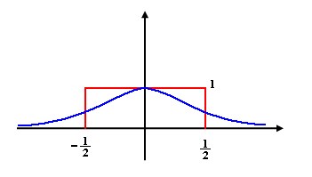
Example of a useful Parzen window function $\in \mathbb{R}^n$

Figure 1 - Useful Parzen Window

\in \mathbb{R}^n

This function has zero mean, H variance, an n-dimensional density, and is not compactly supported.

You can use any $\varphi$ such that:

1) $\varphi(\vec{u})>0,\forall\vec{u}$

2) $\int_{R^n}\varphi(\vec{u})d\vec{u}=1$

Given i samples $\vec{X}_1,\vec{X}_2,...,\vec{X}_i\in{R}^n$ ,

$P_i(\vec{X}_0)=\frac{1}{i\cdot{V}_i}\displaystyle\sum_{l=1}^{i} \varphi(\frac{ \vec{X_l}-\vec{X_0} }{h_i} )$ , where $$ h_i $$ is a number that controls $$ V_i $$ .

i.e. $$ V_i=h_i^n $$ since $V_i=\int\varphi(\frac{\vec{u}}{h_i})d\vec{u}$

Letting $\vec{v}=\frac{\vec{u}}{h_i}$ and $d\vec{v}=\frac{1}{h_i^n}d\vec{u}$ , we have:

$tex: V_i=\int{h_i^n}\varphi(\vec{v})d\vec{v}=h_i^n\int_{R^n}\varphi(\vec{v})d\vec{v}=h_i^n$

$p_1(\vec{X}_0)=\frac{1}{i\cdot{h_i^n}}\displaystyle\sum_{l=1}^{i}\varphi(\frac{\vec{X}_l-\vec{X}_0}{h_i})$ For convergence (in mean square) we need $i\cdot{V_i}\displaystyle\to\infty$ as $i\to\infty$

i.e. $i\cdot{h_i^n}\to\infty$ as $i\to\infty$ , and $h_i\to{0}$ as $i\to\infty$ .

How to make a decision using Parzen window method of density estimation

-> Given samples ${X_1}^j, {X_2}^j ,..., {X_{d_j}}^j$ , for class $$ w_j $$ , i=1,2...,c

The total number of samples for all classes is $$ N $$ .

Choose $$ w_j $$ such that $P(w_j|\vec{x_0}) \geq P(w_i|\vec{x_0})$ , for all i=1,2,...,c

$\Longleftrightarrow p(\vec{x_0}|w_j)P(w_j)\geq p(\vec{x_0}|w_i)P(w_i) \forall i$

$\Longleftrightarrow p(\vec{x_0}, w_j) \geq p(\vec{x_0}, w_i) \forall i$

,where $p(\vec{x_0},w_j) \simeq \frac{1}{N\cdot V} \sum_{l=1}^{d_j}\varphi(\frac{\vec{{x_l}^j}-\vec{x_0}}{h}) \geq \frac{1}{N\cdot V} \sum_{l=1}^{d_i}\varphi(\frac{\vec{{x_l}^i}-\vec{x_0}}{h})$

Therefore, $\sum_{l=1}^{d_j}\varphi(\frac{\vec{x_l^j}-\vec{x_0}}{h}) \geq \sum_{l=1}^{d_i}\varphi(\frac{\vec{x_l^i}-\vec{x_0}}{h})$

In the last equation, the first term represents $$ K_j $$ around $$ x_0 $$ , and the second term represents $$ K_i $$ around $$ x_0 $$ .

"Assign category of majority vote of neighbors", where total # of samples = $\sum_{i=1}^{d}d_i$ .

Observation: Training error can be made=0 (by taking V small enough) but V too small=>spikiness =>high test error

Parzen Window Code

PLEASE HELP FIX THE MATLAB CODE !!!!Parzen Window Estimation example_OldKiwi

Working Parzen Window Code in Scilab_OldKiwi

K-nearest neighbor density estimate

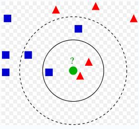
K-Nearest neighbors is a supervised algorithm which basically counts the k-nearest features to determine the class of a sample. The classifiers do not use any model to fit. Given a query, KNN counts the k nearest neighbor points and decide on the class which takes the majority of votes. It is a simple and efficient algorithm that only calculates the distance of a new sample to the nearest neighbors. Assign category based on majority vote of k nearest neighbor. The distance can be chosen as Euclidean distance.

In order to specify the class of green circle, 3-nearest neighbors are counted and because red triangles are more than blue squares, the class of green circle is red triangle.

Assign category based on majority vote of k nearest neighbor

1) Choose region function $\varphi$

for example, hypersphere

$\varphi \left( \frac{\vec{x}-\vec{x_0}}{h} \right)= 1, \qquad ||\frac{\vec{x}-\vec{x_0}}{h}|| <1$ .....(1)

$\quad \quad \qquad =0, \quad else$

Dual to this is the K-nearest neighbors in $$ L_2 $$ sense (Euclidean distance)

hypercube

$\varphi \left( \frac{x-x_0}{h} \right)= 1, \qquad \mid \frac{x-x_0}{h} \mid < \frac{1}{2}$ .....(2)

$\quad \quad \qquad =0, \quad else$ .....(3)

Dual to this is K-nearest neighbor in $L_{\infty}$ sense. Mimi recommended this metric. Why ? ....

If $\varphi$ normal density, there is no dual to this i.e there can not be a metric defined for a gaussian kernel.

2) Pick K

+ k odd, better for 2 category case => no tie vote

+ k=1, same as nearest neighbor decision rule

3) Given $x_0 \in$ feature space and samples $\vec{x_1},\cdots, \vec{x_d}$ , approximate $$ p(x_0) $$ by

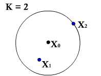
$\bar{p} (x_0)= \frac{K-1}{dV(x_0)}$ => unbiased estimate

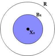
where $$ V(x_0) $$ is volume of smallest region R around $$ x_0 $$ , containing K samples (called prototypes)

or more generally

$\overline{p}\left(x_{0}\right)=\frac{k-\#\, of\, samples\, on\, boundary}{dV(x)}$ .....(4)

this yields,

$E[\bar{p}(x_0)]=p(x_0)$ .....(5)

if $$ p(x_0) $$ where $\frac{K}{dV(x_0)}$ then $E[\bar{p}(x_0)]=\frac{K}{K-1}p(\vec{x}_0)$

Decision rule is still based majority vote

$\frac{K-1}{dV(x_0)} < \frac{K-1}{dV(x)}$ => yields an unbiased estimate

$$ p(x_0) $$ is a random variable

$\bar{p}(x_0)=\frac{K}{dV(x_0)}$ , where $$ V(x_0) $$ is random variable

=> hard to evaluate density of $$ V(x_0) $$

Consider u $u:=\displaystyle \int_{R - B_R} p(x) dx$ .....(6)

where $$ B_R $$ is small band around R

$\Rightarrow u \approx p(x_0) V(x_0)$ .....(7)

$\Delta u = \displaystyle \int _{B_R} p(x) dx$ .....(8)

Let G= event "K-1 samples fall into $$ R- B_R $$ "

and H= event "1 samples falls into band"

$$ p(G,H)=p(G)p(H|G) $$ .....(9)

$p(G)=C^{d}_{k-1} u^{k-1} {(1-u)}^{d-k+1}$ .....(10)

$P(H \mid G)= C^{d-k+1}_{1} \left( \frac{\Delta u}{1-u} \right) { \left( 1- \frac{\Delta u}{1-u} \right) } ^{d-k}$ .....(11)

$C^{d}_{k+1} \left( \frac{d-k+1}{1} \right) \frac{\Delta u}{1-u} u^{k-1} {(1-u)}^{d-k+1} \left( 1- \frac{\Delta u}{1-u} \right)$ .....(12)

keeping the first order term in Taylor approximation

i.e., $\left( 1- \frac{\Delta u}{1-u} \right) \approx 1$ for $\Delta u$ small

$\Rightarrow P(G,H) \approx \Delta u \frac{d!}{(k-1)! (d-k)!} u^{k-1} {(1-u)}^{d-k}$ for $\Delta u$ small

$E[ \bar{p} (x_0)]=E \left[ \frac{k-1}{dV(x_0)} \right] \approx E \left[ \frac{(k-1)}{du} p(x_0) \right] = \displaystyle \int \frac{(k-1)}{du} p(x_0) p_u (u) du = p(x_0)$ .....(13)