| (13 intermediate revisions by 2 users not shown) | |||
| Line 1: | Line 1: | ||
| − | =[[ECE662]] | + | [[Category:ECE662]] |
| + | [[Category:decision theory]] | ||
| + | [[Category:lecture notes]] | ||
| + | [[Category:pattern recognition]] | ||
| + | [[Category:slecture]] | ||
| + | |||
| + | <center><font size= 4> | ||
| + | '''[[ECE662]]: Statistical Pattern Recognition and Decision Making Processes''' | ||
| + | </font size> | ||
| + | |||
| + | Spring 2008, [[user:mboutin|Prof. Boutin]] | ||
| + | |||
| + | [[Slectures|Slecture]] | ||
| + | |||
| + | <font size= 3> Collectively created by the students in [[ECE662:BoutinSpring08_OldKiwi|the class]]</font size> | ||
| + | </center> | ||
| + | |||
| + | ---- | ||
=Lecture 2 Lecture notes= | =Lecture 2 Lecture notes= | ||
| + | Jump to: [[ECE662_Pattern_Recognition_Decision_Making_Processes_Spring2008_sLecture_collective|Outline]]| | ||
| + | [[Lecture 1 - Introduction_OldKiwi|1]]| | ||
| + | [[Lecture 2 - Decision Hypersurfaces_OldKiwi|2]]| | ||
| + | [[Lecture 3 - Bayes classification_OldKiwi|3]]| | ||
| + | [[Lecture 4 - Bayes Classification_OldKiwi|4]]| | ||
| + | [[Lecture 5 - Discriminant Functions_OldKiwi|5]]| | ||
| + | [[Lecture 6 - Discriminant Functions_OldKiwi|6]]| | ||
| + | [[Lecture 7 - MLE and BPE_OldKiwi|7]]| | ||
| + | [[Lecture 8 - MLE, BPE and Linear Discriminant Functions_OldKiwi|8]]| | ||
| + | [[Lecture 9 - Linear Discriminant Functions_OldKiwi|9]]| | ||
| + | [[Lecture 10 - Batch Perceptron and Fisher Linear Discriminant_OldKiwi|10]]| | ||
| + | [[Lecture 11 - Fischer's Linear Discriminant again_OldKiwi|11]]| | ||
| + | [[Lecture 12 - Support Vector Machine and Quadratic Optimization Problem_OldKiwi|12]]| | ||
| + | [[Lecture 13 - Kernel function for SVMs and ANNs introduction_OldKiwi|13]]| | ||
| + | [[Lecture 14 - ANNs, Non-parametric Density Estimation (Parzen Window)_OldKiwi|14]]| | ||
| + | [[Lecture 15 - Parzen Window Method_OldKiwi|15]]| | ||
| + | [[Lecture 16 - Parzen Window Method and K-nearest Neighbor Density Estimate_OldKiwi|16]]| | ||
| + | [[Lecture 17 - Nearest Neighbors Clarification Rule and Metrics_OldKiwi|17]]| | ||
| + | [[Lecture 18 - Nearest Neighbors Clarification Rule and Metrics(Continued)_OldKiwi|18]]| | ||
| + | [[Lecture 19 - Nearest Neighbor Error Rates_OldKiwi|19]]| | ||
| + | [[Lecture 20 - Density Estimation using Series Expansion and Decision Trees_OldKiwi|20]]| | ||
| + | [[Lecture 21 - Decision Trees(Continued)_OldKiwi|21]]| | ||
| + | [[Lecture 22 - Decision Trees and Clustering_OldKiwi|22]]| | ||
| + | [[Lecture 23 - Spanning Trees_OldKiwi|23]]| | ||
| + | [[Lecture 24 - Clustering and Hierarchical Clustering_OldKiwi|24]]| | ||
| + | [[Lecture 25 - Clustering Algorithms_OldKiwi|25]]| | ||
| + | [[Lecture 26 - Statistical Clustering Methods_OldKiwi|26]]| | ||
| + | [[Lecture 27 - Clustering by finding valleys of densities_OldKiwi|27]]| | ||
| + | [[Lecture 28 - Final lecture_OldKiwi|28]] | ||
| + | ---- | ||
---- | ---- | ||
Topic: "Decision hypersurfaces" | Topic: "Decision hypersurfaces" | ||
| Line 6: | Line 53: | ||
Making decisions is the art of drawing hypersurfaces. | Making decisions is the art of drawing hypersurfaces. | ||
| − | The following | + | The following Hypersurfaces are discussed in this lecture: |
* '''Linear Separations''' | * '''Linear Separations''' | ||
| Line 16: | Line 63: | ||
=== Combining Hypersurfaces === | === Combining Hypersurfaces === | ||
| − | + | Hypersurfaces are combined by multiplication of the functions which define them, not by intersection. | |
| − | + | ||
| − | Hypersurfaces are | + | |
=== Tree Based Separation === | === Tree Based Separation === | ||
| Line 59: | Line 104: | ||
===Work in low dimensionality as far as possible=== | ===Work in low dimensionality as far as possible=== | ||
| − | Why? This is typically explained as the [[curse of | + | Why? This is typically explained as the [[Curse_of_Dimensionality_Old_Kiwi|curse of dimensionality]]. For more, this term can be googled. There is a nice [http://citeseer.ist.psu.edu/cache/papers/cs/25919/http:zSzzSzwww.informatik.uni-halle.dezSz~keimzSzPSzSzvldb2000.pdf/hinneburg00what.pdfciteseer| paper] in VLDB 2000 that discusses the notion of nearest-neighbors in high dimensional spaces. |
Let <math>x_{1},x_{2},\ldots,x_{N}</math> be features. Suppose we use a large number of features to come up with a decision hypersurface <math>g(x_{1},x_{2},\ldots,x_{N})=0</math> | Let <math>x_{1},x_{2},\ldots,x_{N}</math> be features. Suppose we use a large number of features to come up with a decision hypersurface <math>g(x_{1},x_{2},\ldots,x_{N})=0</math> | ||
| Line 70: | Line 115: | ||
[[ECE662:BoutinSpring08_OldKiwi|Back to ECE662 Spring 2010]] | [[ECE662:BoutinSpring08_OldKiwi|Back to ECE662 Spring 2010]] | ||
| − | |||
| − | |||
| − | |||
| − | |||
Latest revision as of 11:17, 10 June 2013
ECE662: Statistical Pattern Recognition and Decision Making Processes
Spring 2008, Prof. Boutin
Collectively created by the students in the class
Contents
Lecture 2 Lecture notes
Jump to: Outline| 1| 2| 3| 4| 5| 6| 7| 8| 9| 10| 11| 12| 13| 14| 15| 16| 17| 18| 19| 20| 21| 22| 23| 24| 25| 26| 27| 28
Topic: "Decision hypersurfaces"
Making decisions is the art of drawing hypersurfaces.
The following Hypersurfaces are discussed in this lecture:
- Linear Separations
- Straight lines in 2D $ ax+by+c=0 $
- Planes in 3D $ ax+by+cx+d=0 $
- Hyperplanes in nD $ \sum a_i x_i = \textrm{constant} $
- Union of linear separations
- Tree-based separation
Combining Hypersurfaces
Hypersurfaces are combined by multiplication of the functions which define them, not by intersection.
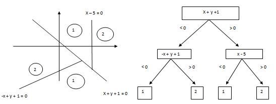
Tree Based Separation
By using union of hypersurfaces, classes can be separated by a tree based structure. Tree based separation is harder, and obtaining an optimum decision tree is another difficult problem in pattern recognition.
Example:
Question: What do we mean by good separation?
Question: What do we mean by good separation?
Meaning 1: One that will make few mistakes when used to classify actual data. In statistical language: small probability of error.
Meaning 2: One that will make mistakes that will not be too costly. In statistical language: small expected cost of errors.
Note
If the cost function $ c(x) $ from Meaning 2 is defined to be 1 for an error, and 0 otherwise, then $ E[c(x)] = P[error] $, so that Meaning 1 is a special case of Meaning 2.
Illustration
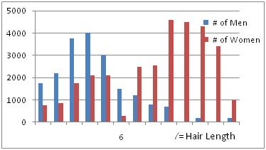
Take 50,000 people in an airport. We want to be able to distinguish men from women among these 50,000 people.
Use hairlength as the single feature.
Histogram represents the actual numbers.
Decision hypersurface: $ l-6=0 $. This is the best decision rule in the sense that it minimizes the probability of error. Can not do better than this for the scenario where only hairlength is used as the feature.
Remember
- Good features produce distinct bumps. That is try to choose features that have a natural grouping for a particular class. For example, hair-length is a good feature to separate men from women as more most men are likely to have short hair-length.
- Bad features (e.g. background color) produce overlapping bumps.
- In order to get a good decision algorithm, we need to have good features (and good separation too).
Work in low dimensionality as far as possible
Why? This is typically explained as the curse of dimensionality. For more, this term can be googled. There is a nice paper in VLDB 2000 that discusses the notion of nearest-neighbors in high dimensional spaces.
Let $ x_{1},x_{2},\ldots,x_{N} $ be features. Suppose we use a large number of features to come up with a decision hypersurface $ g(x_{1},x_{2},\ldots,x_{N})=0 $
Then g is the single feature we need.


