(→PDE based valley seeking) |
|||
| (34 intermediate revisions by 7 users not shown) | |||
| Line 1: | Line 1: | ||
| + | [[Category:ECE662]] | ||
| + | [[Category:decision theory]] | ||
| + | [[Category:lecture notes]] | ||
| + | [[Category:pattern recognition]] | ||
| + | [[Category:slecture]] | ||
| + | <center><font size= 4> | ||
| + | '''[[ECE662]]: Statistical Pattern Recognition and Decision Making Processes''' | ||
| + | </font size> | ||
| + | |||
| + | Spring 2008, [[user:mboutin|Prof. Boutin]] | ||
| + | |||
| + | [[Slectures|Slecture]] | ||
| + | |||
| + | <font size= 3> Collectively created by the students in [[ECE662:BoutinSpring08_OldKiwi|the class]]</font size> | ||
| + | </center> | ||
| + | |||
| + | ---- | ||
| + | =Lecture 27 Lecture notes= | ||
| + | Jump to: [[ECE662_Pattern_Recognition_Decision_Making_Processes_Spring2008_sLecture_collective|Outline]]| | ||
| + | [[Lecture 1 - Introduction_OldKiwi|1]]| | ||
| + | [[Lecture 2 - Decision Hypersurfaces_OldKiwi|2]]| | ||
| + | [[Lecture 3 - Bayes classification_OldKiwi|3]]| | ||
| + | [[Lecture 4 - Bayes Classification_OldKiwi|4]]| | ||
| + | [[Lecture 5 - Discriminant Functions_OldKiwi|5]]| | ||
| + | [[Lecture 6 - Discriminant Functions_OldKiwi|6]]| | ||
| + | [[Lecture 7 - MLE and BPE_OldKiwi|7]]| | ||
| + | [[Lecture 8 - MLE, BPE and Linear Discriminant Functions_OldKiwi|8]]| | ||
| + | [[Lecture 9 - Linear Discriminant Functions_OldKiwi|9]]| | ||
| + | [[Lecture 10 - Batch Perceptron and Fisher Linear Discriminant_OldKiwi|10]]| | ||
| + | [[Lecture 11 - Fischer's Linear Discriminant again_OldKiwi|11]]| | ||
| + | [[Lecture 12 - Support Vector Machine and Quadratic Optimization Problem_OldKiwi|12]]| | ||
| + | [[Lecture 13 - Kernel function for SVMs and ANNs introduction_OldKiwi|13]]| | ||
| + | [[Lecture 14 - ANNs, Non-parametric Density Estimation (Parzen Window)_OldKiwi|14]]| | ||
| + | [[Lecture 15 - Parzen Window Method_OldKiwi|15]]| | ||
| + | [[Lecture 16 - Parzen Window Method and K-nearest Neighbor Density Estimate_OldKiwi|16]]| | ||
| + | [[Lecture 17 - Nearest Neighbors Clarification Rule and Metrics_OldKiwi|17]]| | ||
| + | [[Lecture 18 - Nearest Neighbors Clarification Rule and Metrics(Continued)_OldKiwi|18]]| | ||
| + | [[Lecture 19 - Nearest Neighbor Error Rates_OldKiwi|19]]| | ||
| + | [[Lecture 20 - Density Estimation using Series Expansion and Decision Trees_OldKiwi|20]]| | ||
| + | [[Lecture 21 - Decision Trees(Continued)_OldKiwi|21]]| | ||
| + | [[Lecture 22 - Decision Trees and Clustering_OldKiwi|22]]| | ||
| + | [[Lecture 23 - Spanning Trees_OldKiwi|23]]| | ||
| + | [[Lecture 24 - Clustering and Hierarchical Clustering_OldKiwi|24]]| | ||
| + | [[Lecture 25 - Clustering Algorithms_OldKiwi|25]]| | ||
| + | [[Lecture 26 - Statistical Clustering Methods_OldKiwi|26]]| | ||
| + | [[Lecture 27 - Clustering by finding valleys of densities_OldKiwi|27]]| | ||
| + | [[Lecture 28 - Final lecture_OldKiwi|28]] | ||
| + | ---- | ||
| + | ---- | ||
== Clustering by finding valleys of densities == | == Clustering by finding valleys of densities == | ||
| + | -- Approach 1: "Bump Hunting" -- | ||
| + | - Approximate p(x) | ||
| + | - Find peaks of density | ||
| + | - Expand cluster boundaries outward until they meet (hopefully in middle!) | ||
| + | - Define meeting points = Cluster boundary points | ||
| + | |||
| + | [[Image:Lec27_fig1_OldKiwi.GIF]] (fig.1) | ||
| + | |||
| + | -- Approach 2: "Valley Seeking" -- | ||
| + | - Start from valley regions of p(x) | ||
| + | - Work uphill to connect data points to density peaks | ||
| + | |||
| + | [[Image:Lec27_fig2_OldKiwi.GIF]] (fig.2) | ||
== Graph based implementation == | == Graph based implementation == | ||
| + | - Estimate p(x) | ||
| + | - For all patterns <math>X_i</math>, denote by <math>N_r(X_i)</math>, the neighborhood of size <math>r</math> of <math>X_i</math>. | ||
| + | - Estimate derivative of density p(x) along direction <math>X_i-X_j, \forall X_j\in N_r(X_i)</math> | ||
| + | <math>S_i(j)=\frac{p(X_i)-p(X_j)}{||X_i-X_j||_{L_2}}</math> | ||
| + | Let <math>j_{max}=argmax_j S_i(j)</math> | ||
| + | If <math>S_i(j_{max})<0</math> declare <math>i</math> to be a root node. | ||
| + | If <math>S_i(j_{max})>0</math> declare <math>X_{j_{max}}</math> to be parent of <math>X_i</math>. | ||
| + | If <math>S_i(j_{max})=0</math> it depends on the surroundings what link we establish. | ||
| + | - If <math>X_i</math> is connected to a root node, then make this root node a parent of <math>X_i</math>, else make <math>X_i</math> a root node. | ||
| + | - Repeat | ||
| + | When all points are visited, a forest is constructed. Each connected component (=tree of a forest) is a cluster. | ||
| + | |||
| + | * Problem: All methods presented above encounter a serious problem because of the following reasons: | ||
| + | |||
| + | - Density may oscillate a lot | ||
| + | - Valleys are not well defined. | ||
| + | |||
| + | [[Image:Lec27_fig3_OldKiwi.GIF]](fig.3) | ||
== PDE based valley seeking == | == PDE based valley seeking == | ||
| Line 15: | Line 95: | ||
Consider 1-D curves | Consider 1-D curves | ||
| − | <math>u(x): [0,1] \rightarrow \Re</math> with fixed end points u(0)=a, u(1)=b (3-1) | + | <math>u(x): [0,1] \rightarrow \Re</math> with fixed end points <math>u(0)=a</math>, <math>u(1)=b</math> (3-1) |
| − | + | [[Image:Park211_OldKiwi.jpg]] | |
Suppose Energy of curve is | Suppose Energy of curve is | ||
| Line 29: | Line 109: | ||
sometimes written as <math>E'=0 \Rightarrow \frac{\partial E}{\partial u}=0</math> (3-4) | sometimes written as <math>E'=0 \Rightarrow \frac{\partial E}{\partial u}=0</math> (3-4) | ||
| + | |||
| + | |||
Similarly if <math>E=\int _0 ^1 F(u,u',u'')dx</math> (3-5) | Similarly if <math>E=\int _0 ^1 F(u,u',u'')dx</math> (3-5) | ||
| Line 34: | Line 116: | ||
e.g.) <math>F(u,u',u'')=|u''|^2</math> (3-6) | e.g.) <math>F(u,u',u'')=|u''|^2</math> (3-6) | ||
| − | Then Euler equation is <math>\frac{\partial F}{\partial u} - \frac{d}{dx}(\frac{\partial F}{\partial u'}) + \frac{d}{dx^2}(\frac{\partial F}{\partial u''})=0</math> (3-7) | + | Then Euler equation is <math>\frac{\partial F}{\partial u} - \frac{d}{dx}(\frac{\partial F}{\partial u'}) + \frac{d^2}{dx^2}(\frac{\partial F}{\partial u''})=0</math> (3-7) |
Similarly, for surface in <math>\Re ^2</math> | Similarly, for surface in <math>\Re ^2</math> | ||
| Line 46: | Line 128: | ||
e.g.) <math>F={u_x}^2+{u_y}^2</math> (3-10) | e.g.) <math>F={u_x}^2+{u_y}^2</math> (3-10) | ||
| − | Then Euler equation is | + | Then Euler equation is |
| + | |||
| + | <math>\frac{\partial F}{\partial u} - \frac{d}{dx}(\frac{\partial F}{\partial u_x}) - \frac{d}{dy}(\frac{\partial F}{\partial u_y}) + \frac{d^2}{dx^2}(\frac{\partial F}{\partial u_{xx}}) + \frac{d^2}{dy^2}(\frac{\partial F}{\partial u_{yy}}) + \frac{d^2}{dxdy}(\frac{\partial F}{\partial u_{xy}})=0</math> (3-11) | ||
| + | |||
| + | * Illustration | ||
| + | |||
| + | 1D curve <math>u(x)</math> with <math>u(0)=a, u(1)=b</math> (3-12) | ||
| + | |||
| + | <math>E(u)=\int _{0} ^{1} ||\nabla u||^2 dx</math> (3-13) Dirichlet integral | ||
| + | |||
| + | <math>F=||\nabla u||^2=u_x ^2</math> | ||
| + | |||
| + | Euler equation E'=0 | ||
| + | |||
| + | <math>\frac{\partial F}{\partial u} - \frac{d}{dx}(\frac{\partial F}{\partial u_x})=0 </math> (3-14) | ||
| + | |||
| + | <math>0-\frac{d}{dx}(2u_x)=0 \Rightarrow -2u_{xx}=0 \Rightarrow u_{xx}=0</math> (3-15) | ||
| + | |||
| + | with boundary condition, <math>u(0)=0, u(1)=b</math> | ||
| + | |||
| + | Solution: <math>u(x)=c_1 x+ c_2</math> | ||
| + | |||
| + | <math>u(0)=a \Rightarrow c_2=a</math> (3-16) | ||
| + | |||
| + | <math>u(1)=b \Rightarrow c_1 + c_2 = b \Rightarrow c_1=b-a</math> (3-17) | ||
| + | |||
| + | [[Image:park212_OldKiwi.jpg]] | ||
| + | |||
| + | In general, cannot solve Euler equation analytically | ||
| + | |||
| + | In practice, use 'Gradient descent' | ||
| + | |||
| + | Pick initial curve <math>u_0 (x)</math> | ||
| + | |||
| + | Consider a family of curves <math>u(t,x)</math> such that <math>u(0,x)=u_0 (x)</math> and <math>\frac{\partial u}{\partial t}= \pm E'</math> (3-18) | ||
| + | |||
| + | +: if looking for max | ||
| + | |||
| + | -: if looking for min | ||
| + | |||
| + | t is called "time marching parameter" | ||
| + | |||
| + | Solve for <math>u(t,x)</math> numerically, when "steady state" <math>\frac{\partial u}{\partial E}=0</math> is achieved. (3-19) | ||
| + | |||
| + | Say at <math>u(t_{final},x)=: u_1 (x)</math> (3-20) | ||
| + | |||
| + | Then <math>u_1(x)</math> is the solution to Euler Equation <math>E'=0</math> | ||
| + | |||
| + | *Example | ||
| + | |||
| + | <math>F=||\nabla u||^2 = u_x ^2</math> (3-21) | ||
| + | |||
| + | Look for curve <math>u(x)</math> such that <math>u(0)=a, u(1)=b</math> with minimum E. (3-22) | ||
| + | |||
| + | Consider <math>u(t,x)</math> | ||
| + | |||
| + | <math>u(0,x)</math> is initial guess | ||
| + | |||
| + | Gradient descent (Equation to Euler's equation) | ||
| + | |||
| + | <math>\frac{\partial u}{\partial t}=u_{xx}</math> "Heat Equation" (3-23) | ||
| + | |||
| + | <<Picture>> | ||
| + | |||
| + | * curve gets less and less curvy as t evolves | ||
| + | * in fact, evolving for t units is equivalent to convolving <math>u_0 (x)</math> with Gaussian kernel | ||
| + | |||
| + | <math>G(x,t)=\sqrt{\frac{1}{4 \pi t}} e^{-\frac{x^2}{4t}}</math> (3-24) | ||
| + | |||
| + | i.e., <math>u(t,x)=u_0 (x) * G(x,t)</math> | ||
| + | |||
| + | <<Figure>> | ||
| + | |||
| + | Scale space of curves | ||
| + | |||
| + | [[Image:ECE662 lect27 smear_OldKiwi.gif]] | ||
| + | |||
| + | If cannot solve <math>\frac{\partial u}{\partial t}=E'</math> discretize and solve numerically (3-25) | ||
| + | |||
| + | <math>\frac{\partial u}{\partial t} \approx \frac{u(t+ | ||
| + | \Delta t ,x )-u(t,x)}{\Delta t}</math> (3-26) | ||
| + | |||
| + | <math>u_{xx} \approx \frac{u(t,x+\Delta x)-2u(t,x)+u(t,x-\Delta x)}{\Delta x^2}</math> (3-27) | ||
| + | |||
| + | <math>\frac{\partial u}{\partial t}=u_{xx}</math> (3-28) | ||
| + | |||
| + | <math>\frac{u(t+\Delta t,x)-u(t,x)}{\Delta t}=\frac{u(t,x+\Delta x)-2u(t,x)+u(t,x-\Delta x)}{\Delta x^2}</math> (3-29) | ||
| + | |||
| + | <math>u(t+\Delta t, x)=u(t,x)+\frac{\Delta t}{\Delta x^2}(u(t,x+\Delta x)-2u(t,x)+u(t,x-\Delta x))</math> (3-30) | ||
Latest revision as of 11:24, 10 June 2013
ECE662: Statistical Pattern Recognition and Decision Making Processes
Spring 2008, Prof. Boutin
Collectively created by the students in the class
Contents
Lecture 27 Lecture notes
Jump to: Outline| 1| 2| 3| 4| 5| 6| 7| 8| 9| 10| 11| 12| 13| 14| 15| 16| 17| 18| 19| 20| 21| 22| 23| 24| 25| 26| 27| 28
Clustering by finding valleys of densities
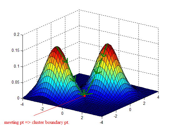
-- Approach 1: "Bump Hunting" --
   - Approximate p(x)
   - Find peaks of density
   - Expand cluster boundaries outward until they meet (hopefully in middle!)
   - Define meeting points = Cluster boundary points
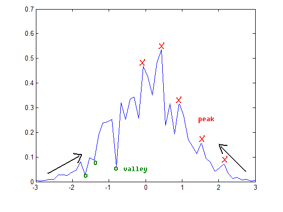
-- Approach 2: "Valley Seeking" --
   - Start from valley regions of p(x)
   - Work uphill to connect data points to density peaks
Graph based implementation
   - Estimate p(x)
   - For all patterns $ X_i $, denote by $ N_r(X_i) $, the neighborhood of size $ r $ of $ X_i $.
   - Estimate derivative of density p(x) along direction $ X_i-X_j, \forall X_j\in N_r(X_i) $
           $ S_i(j)=\frac{p(X_i)-p(X_j)}{||X_i-X_j||_{L_2}} $
           Let $ j_{max}=argmax_j S_i(j) $
           If $ S_i(j_{max})<0 $ declare $ i $ to be a root node.
           If $ S_i(j_{max})>0 $ declare $ X_{j_{max}} $ to be parent of $ X_i $.
           If $ S_i(j_{max})=0 $ it depends on the surroundings what link we establish.
   - If $ X_i $ is connected to a root node, then make this root node a parent of $ X_i $, else make $ X_i $ a root node.
   - Repeat
When all points are visited, a forest is constructed. Each connected component (=tree of a forest) is a cluster.
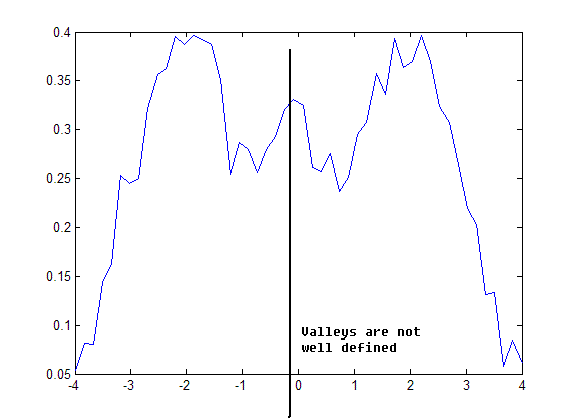
- Problem: All methods presented above encounter a serious problem because of the following reasons:
   - Density may oscillate a lot
   - Valleys are not well defined.
PDE based valley seeking
PDE: Partial Differential Equation
PDE's can be used to minimize energy functionals
- Simple Example
Consider 1-D curves
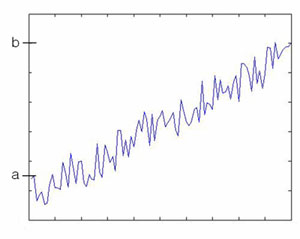
$ u(x): [0,1] \rightarrow \Re $ with fixed end points $ u(0)=a $, $ u(1)=b $ (3-1)
Suppose Energy of curve is $ E(u)=\int _0 ^1 F(u, u')dx $ for some function $ F: \Re ^2 \rightarrow \Re $
e.g.) $ F(u,u')=|u'|^2 $ (3-2)
The curve that minimizes (or maximizes) E(u) satisfies Euler Equation
$ \frac{\partial F} {\partial u} -\frac{d}{dx}(\frac{\partial F}{\partial u'})=0 $ (3-3)
sometimes written as $ E'=0 \Rightarrow \frac{\partial E}{\partial u}=0 $ (3-4)
Similarly if $ E=\int _0 ^1 F(u,u',u'')dx $ (3-5)
e.g.) $ F(u,u',u'')=|u''|^2 $ (3-6)
Then Euler equation is $ \frac{\partial F}{\partial u} - \frac{d}{dx}(\frac{\partial F}{\partial u'}) + \frac{d^2}{dx^2}(\frac{\partial F}{\partial u''})=0 $ (3-7)
Similarly, for surface in $ \Re ^2 $
$ u(x,y): [0,1] \times [0,1] \rightarrow \Re $ (3-8)
Suppose energy is given by
$ E(u)=\int _{surface} F(u,u_x, u_y, u_{xx}, u_{xy},u_{yy})dxdy $ (3-9)
e.g.) $ F={u_x}^2+{u_y}^2 $ (3-10)
Then Euler equation is
$ \frac{\partial F}{\partial u} - \frac{d}{dx}(\frac{\partial F}{\partial u_x}) - \frac{d}{dy}(\frac{\partial F}{\partial u_y}) + \frac{d^2}{dx^2}(\frac{\partial F}{\partial u_{xx}}) + \frac{d^2}{dy^2}(\frac{\partial F}{\partial u_{yy}}) + \frac{d^2}{dxdy}(\frac{\partial F}{\partial u_{xy}})=0 $ (3-11)
- Illustration
1D curve $ u(x) $ with $ u(0)=a, u(1)=b $ (3-12)
$ E(u)=\int _{0} ^{1} ||\nabla u||^2 dx $ (3-13) Dirichlet integral
$ F=||\nabla u||^2=u_x ^2 $
Euler equation E'=0
$ \frac{\partial F}{\partial u} - \frac{d}{dx}(\frac{\partial F}{\partial u_x})=0 $ (3-14)
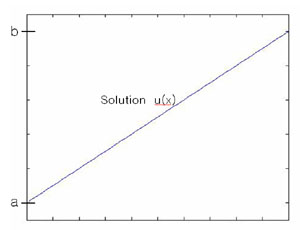
$ 0-\frac{d}{dx}(2u_x)=0 \Rightarrow -2u_{xx}=0 \Rightarrow u_{xx}=0 $ (3-15)
with boundary condition, $ u(0)=0, u(1)=b $
Solution: $ u(x)=c_1 x+ c_2 $
$ u(0)=a \Rightarrow c_2=a $ (3-16)
$ u(1)=b \Rightarrow c_1 + c_2 = b \Rightarrow c_1=b-a $ (3-17)
In general, cannot solve Euler equation analytically
In practice, use 'Gradient descent'
Pick initial curve $ u_0 (x) $
Consider a family of curves $ u(t,x) $ such that $ u(0,x)=u_0 (x) $ and $ \frac{\partial u}{\partial t}= \pm E' $ (3-18)
+: if looking for max
-: if looking for min
t is called "time marching parameter"
Solve for $ u(t,x) $ numerically, when "steady state" $ \frac{\partial u}{\partial E}=0 $ is achieved. (3-19)
Say at $ u(t_{final},x)=: u_1 (x) $ (3-20)
Then $ u_1(x) $ is the solution to Euler Equation $ E'=0 $
- Example
$ F=||\nabla u||^2 = u_x ^2 $ (3-21)
Look for curve $ u(x) $ such that $ u(0)=a, u(1)=b $ with minimum E. (3-22)
Consider $ u(t,x) $
$ u(0,x) $ is initial guess
Gradient descent (Equation to Euler's equation)
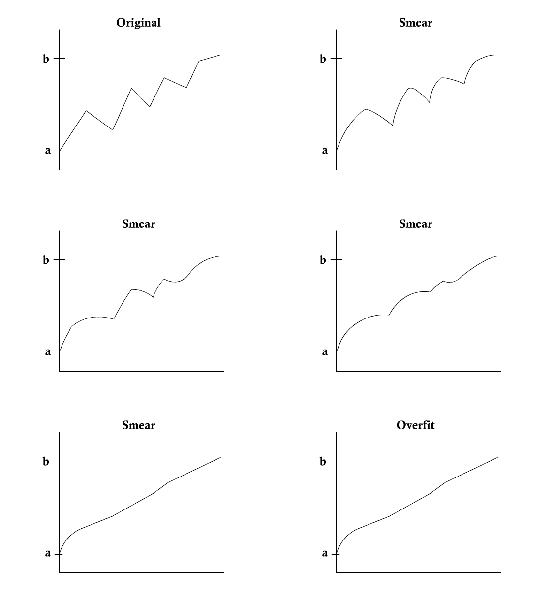
$ \frac{\partial u}{\partial t}=u_{xx} $ "Heat Equation" (3-23)
<<Picture>>
- curve gets less and less curvy as t evolves
- in fact, evolving for t units is equivalent to convolving $ u_0 (x) $ with Gaussian kernel
$ G(x,t)=\sqrt{\frac{1}{4 \pi t}} e^{-\frac{x^2}{4t}} $ (3-24)
i.e., $ u(t,x)=u_0 (x) * G(x,t) $
<<Figure>>
Scale space of curves
If cannot solve $ \frac{\partial u}{\partial t}=E' $ discretize and solve numerically (3-25)
$ \frac{\partial u}{\partial t} \approx \frac{u(t+ \Delta t ,x )-u(t,x)}{\Delta t} $ (3-26)
$ u_{xx} \approx \frac{u(t,x+\Delta x)-2u(t,x)+u(t,x-\Delta x)}{\Delta x^2} $ (3-27)
$ \frac{\partial u}{\partial t}=u_{xx} $ (3-28)
$ \frac{u(t+\Delta t,x)-u(t,x)}{\Delta t}=\frac{u(t,x+\Delta x)-2u(t,x)+u(t,x-\Delta x)}{\Delta x^2} $ (3-29)
$ u(t+\Delta t, x)=u(t,x)+\frac{\Delta t}{\Delta x^2}(u(t,x+\Delta x)-2u(t,x)+u(t,x-\Delta x)) $ (3-30)

