| (35 intermediate revisions by 8 users not shown) | |||
| Line 1: | Line 1: | ||
| − | [ | + | <center><font size= 4> |
| + | '''[[ECE662]]: Statistical Pattern Recognition and Decision Making Processes''' | ||
| + | </font size> | ||
| − | [ | + | Spring 2008, [[user:mboutin|Prof. Boutin]] |
| − | + | [[Slectures|Slecture]] | |
| − | + | ||
| − | + | <font size= 3> Collectively created by the students in [[ECE662:BoutinSpring08_OldKiwi|the class]]</font size> | |
| + | </center> | ||
| − | + | ---- | |
| − | + | =Lecture 18 Lecture notes= | |
| − | + | Jump to: [[ECE662_Pattern_Recognition_Decision_Making_Processes_Spring2008_sLecture_collective|Outline]]| | |
| + | [[Lecture 1 - Introduction_OldKiwi|1]]| | ||
| + | [[Lecture 2 - Decision Hypersurfaces_OldKiwi|2]]| | ||
| + | [[Lecture 3 - Bayes classification_OldKiwi|3]]| | ||
| + | [[Lecture 4 - Bayes Classification_OldKiwi|4]]| | ||
| + | [[Lecture 5 - Discriminant Functions_OldKiwi|5]]| | ||
| + | [[Lecture 6 - Discriminant Functions_OldKiwi|6]]| | ||
| + | [[Lecture 7 - MLE and BPE_OldKiwi|7]]| | ||
| + | [[Lecture 8 - MLE, BPE and Linear Discriminant Functions_OldKiwi|8]]| | ||
| + | [[Lecture 9 - Linear Discriminant Functions_OldKiwi|9]]| | ||
| + | [[Lecture 10 - Batch Perceptron and Fisher Linear Discriminant_OldKiwi|10]]| | ||
| + | [[Lecture 11 - Fischer's Linear Discriminant again_OldKiwi|11]]| | ||
| + | [[Lecture 12 - Support Vector Machine and Quadratic Optimization Problem_OldKiwi|12]]| | ||
| + | [[Lecture 13 - Kernel function for SVMs and ANNs introduction_OldKiwi|13]]| | ||
| + | [[Lecture 14 - ANNs, Non-parametric Density Estimation (Parzen Window)_OldKiwi|14]]| | ||
| + | [[Lecture 15 - Parzen Window Method_OldKiwi|15]]| | ||
| + | [[Lecture 16 - Parzen Window Method and K-nearest Neighbor Density Estimate_OldKiwi|16]]| | ||
| + | [[Lecture 17 - Nearest Neighbors Clarification Rule and Metrics_OldKiwi|17]]| | ||
| + | [[Lecture 18 - Nearest Neighbors Clarification Rule and Metrics(Continued)_OldKiwi|18]]| | ||
| + | [[Lecture 19 - Nearest Neighbor Error Rates_OldKiwi|19]]| | ||
| + | [[Lecture 20 - Density Estimation using Series Expansion and Decision Trees_OldKiwi|20]]| | ||
| + | [[Lecture 21 - Decision Trees(Continued)_OldKiwi|21]]| | ||
| + | [[Lecture 22 - Decision Trees and Clustering_OldKiwi|22]]| | ||
| + | [[Lecture 23 - Spanning Trees_OldKiwi|23]]| | ||
| + | [[Lecture 24 - Clustering and Hierarchical Clustering_OldKiwi|24]]| | ||
| + | [[Lecture 25 - Clustering Algorithms_OldKiwi|25]]| | ||
| + | [[Lecture 26 - Statistical Clustering Methods_OldKiwi|26]]| | ||
| + | [[Lecture 27 - Clustering by finding valleys of densities_OldKiwi|27]]| | ||
| + | [[Lecture 28 - Final lecture_OldKiwi|28]] | ||
| + | ---- | ||
| + | ---- | ||
| + | == Nearest Neighbors Classification Rule (Alternative Approach) == | ||
| − | Do | + | * Find invariant coordinates |
| + | <math>\varphi : \Re ^k \rightarrow \Re ^n </math> | ||
| + | such that <math>\varphi (x) = \varphi (\bar x) </math> for all <math>x, \bar x</math> which are related by a rotation & translation | ||
| + | Do NOT trivialize! | ||
| − | + | '''Example:''' <math>\varphi (x) =0 </math> gives us a trivial invariant coordinate. But, you lose information about separation, since everything is mapped to zero. | |
Want <math>\varphi (x) = \varphi (\bar x) </math> | Want <math>\varphi (x) = \varphi (\bar x) </math> | ||
<math>\Leftrightarrow x, \bar x</math> are related by a rotation and translation | <math>\Leftrightarrow x, \bar x</math> are related by a rotation and translation | ||
| − | Example | + | '''Example:''' |
<math>p=(p_1,p_2,\cdots, p_N) \in \Re ^{3 \times N}</math> | <math>p=(p_1,p_2,\cdots, p_N) \in \Re ^{3 \times N}</math> | ||
| − | <math>\varphi</math> maps representation position of | + | <math>\varphi</math> maps representation position of tags on body onto <math>(d_{12},d_{13},d_{14},\cdots , d_{N-1, N} )</math> |
| − | + | ||
where <math>d_{ij}</math>= Euclidean distance between <math>p_i</math> and <math>p_j</math> | where <math>d_{ij}</math>= Euclidean distance between <math>p_i</math> and <math>p_j</math> | ||
| − | + | In the above example, we can reconstruct up to a rotation and translation. | |
| − | + | WARNING: Euclidean distance in the invariant coordinate space has nothing to do with Euclidean distance or Procrustes distance in initial feature space. | |
| − | Nearest Neighbor in <math>\Re ^2</math> yields | + | Nearest Neighbor in <math>\Re ^2</math> yields tessellation (tiling of floor with 2D shapes such that 1) no holes and 2) cover all of <math>\Re ^2</math> ). The tessellations separate sample space into regions. Shape of cells depends on metric chosen. See Figure 1. |
| − | |||
| − | + | <center>[[Image:Tessellation_OldKiwi.jpg|frame|Figure 1 - Separation of Sample Space using Tessellations]]</center> | |
| − | < | + | |
| − | Instead of working with (x,y) rotationally invariant, work with <math>z=\sqrt{x^2 + y^2}</math> | + | |
| + | <center>[[Image:lec18_nn_r2_OldKiwi.PNG|frame|Figure 1b - Tessellations]]</center> | ||
| + | |||
| + | |||
| + | '''Example:''' if feature vectors are such that vectors related by a rotation belong to same class | ||
| + | <math>\rightarrow</math> metric should be chosen so that tiles are rotationally symmetric. See Figure 2. | ||
| + | |||
| + | |||
| + | <center>[[Image:Rotation_OldKiwi.jpg|frame|Figure 2 - Example of Vectors related by Rotations]]</center> | ||
| + | |||
| + | |||
| + | Instead of working with (x,y) rotationally invariant, work with <math>z=\sqrt{x^2 + y^2}</math> (distance from origin) | ||
How good is Nearest Neighbor rule? | How good is Nearest Neighbor rule? | ||
| − | + | # Training error is zero: does not measure the "goodness" of a rule | |
| − | + | # Test error: want it to be equal to Bayes error rate, because this yields the minimum error | |
---- | ---- | ||
| − | + | == Nearest Neighbor error rate == | |
| − | + | ||
| + | '''Recall:''' | ||
Probability of error (error rate) on test data is | Probability of error (error rate) on test data is | ||
<math>P(e)=\int p(e \mid \vec{x}) p(\vec{x}) d\vec{x}</math> | <math>P(e)=\int p(e \mid \vec{x}) p(\vec{x}) d\vec{x}</math> | ||
| Line 53: | Line 98: | ||
Let <math>P=\lim_{d \rightarrow \infty } P_{d}(e) </math> | Let <math>P=\lim_{d \rightarrow \infty } P_{d}(e) </math> | ||
| − | Claim | + | '''Claim:''' limit error rate <math>P=\int (1-\sum _{i=1} ^{c}p^2 (\omega _i \mid \vec{x}))p(x)dx</math> |
| − | limit error rate <math>P=\int (1-\sum _{i=1} ^{c}p^2 (\omega _i \mid \vec{x}))p(x)dx</math> | + | |
| − | Proof of claim: Given observation <math>\vec{x}</math>, denode by <math>\vec{x'}_d</math> the nearest neighbor of <math>\vec{x}</math> among <math>\{\vec{x}_1,\vec{x}_2, \cdots , \vec{x}_d \}</math> | + | '''Proof of claim:''' Given observation <math>\vec{x}</math>, denode by <math>\vec{x'}_d</math> the nearest neighbor of <math>\vec{x}</math> among <math>\{\vec{x}_1,\vec{x}_2, \cdots , \vec{x}_d \}</math> |
| − | <math>P_d(e \mid \vec{x})=\int p_d(e \mid \vec{x}, \vec{x}_d)p_d(\vec{x'}_d \mid \vec{x})</math> | + | <math>P_d(e \mid \vec{x})=\int p_d(e \mid \vec{x}, \vec{x'}_d)p_d(\vec{x'}_d \mid \vec{x})p(x)dx</math> |
| − | but <math>\lim _{d \rightarrow \infty } p_d (\vec{x'}_d \mid \vec{x})=\delta {\vec{x'}-\vec{x}}</math> | + | but <math>\lim _{d \rightarrow \infty } p_d (\vec{x'}_d \mid \vec{x})=\delta ({\vec{x' _d }-\vec{x}})</math> |
because probability that sample falls into region R centered at <math>\vec{x}</math> is <math>P_{R}=\int _R p(\vec{x' _d})d \vec{x'}_d</math>. | because probability that sample falls into region R centered at <math>\vec{x}</math> is <math>P_{R}=\int _R p(\vec{x' _d})d \vec{x'}_d</math>. | ||
| Line 68: | Line 112: | ||
So, <math>\lim _{d \rightarrow \infty} \vec{x'}_d = \vec{x}</math> and <math>p_d (\vec{x'}_d \mid \vec{x})=\delta (\vec{x'}_d -\vec{x})+\epsilon _d (\vec{x})</math> where <math>\lim _{d \rightarrow \infty } \epsilon _d (x)=0</math> | So, <math>\lim _{d \rightarrow \infty} \vec{x'}_d = \vec{x}</math> and <math>p_d (\vec{x'}_d \mid \vec{x})=\delta (\vec{x'}_d -\vec{x})+\epsilon _d (\vec{x})</math> where <math>\lim _{d \rightarrow \infty } \epsilon _d (x)=0</math> | ||
| − | Now <math>p_d (e \mid \vec{x}, \vec{x'}_d)</math> ? | + | Now <math>p_d (e \mid \vec{x}, \vec{x'}_d)</math> = ? |
Let <math>\theta , \theta _1 , \theta _2 , \cdots, \theta _{d}</math> be the class of <math>x , x_1 , x_2 , \cdots , x_d</math>, respectively. | Let <math>\theta , \theta _1 , \theta _2 , \cdots, \theta _{d}</math> be the class of <math>x , x_1 , x_2 , \cdots , x_d</math>, respectively. | ||
| Line 74: | Line 118: | ||
Using nearest neighbor rule, error if <math>\theta \neq</math>class of <math> \vec{x'}_d</math><math>=: \theta ' _d</math> | Using nearest neighbor rule, error if <math>\theta \neq</math>class of <math> \vec{x'}_d</math><math>=: \theta ' _d</math> | ||
| − | <math>\Rightarrow | + | <math>\Rightarrow p_d(e \mid \vec{x},\vec{x'}_d)=1-\sum_{i=1} ^ c p(\theta = \omega _i , \theta ' _d = \omega _i \mid \vec{x}, \vec{x'}_d )</math> |
<math>=1- \sum _{i=1} ^c p(\omega _i \mid \vec{x}) p(\omega _i \mid \vec{x'} _d) </math> | <math>=1- \sum _{i=1} ^c p(\omega _i \mid \vec{x}) p(\omega _i \mid \vec{x'} _d) </math> | ||
| − | Recall <math> | + | Recall <math>p_d (e \mid \vec{x}, \vec{x'}_d)p_d (\vec{x'}_d \mid \vec{x})d \vec{x'}_d</math> |
| − | + | You get: <math>p_d (e \mid \vec{x})=(1-\sum _{i=1} ^c p(\omega _i \mid x) p(\omega _i \mid x) )</math> + {something that goes to zero as d goes to <math>\infty</math>} | |
| − | + | ||
<math>\lim _{d \rightarrow \infty} p_d (e \mid \vec{x})=(1- \sum _{i=1} ^c {p(\omega _i \mid x)}^2)</math> | <math>\lim _{d \rightarrow \infty} p_d (e \mid \vec{x})=(1- \sum _{i=1} ^c {p(\omega _i \mid x)}^2)</math> | ||
| − | --[[ | + | ---- |
| + | Previous: [[Lecture_17_-_Nearest_Neighbors_Clarification_Rule_and_Metrics_OldKiwi|Lecture 17]] | ||
| + | Next: [[Lecture_19_-_Nearest_Neighbor_Error_Rates_OldKiwi|Lecture 19]] | ||
| + | |||
| + | [[ECE662:BoutinSpring08_OldKiwi|Back to ECE662 Spring 2008 Prof. Boutin]] | ||
| + | [[Category:ECE662]] | ||
| + | [[Category:decision theory]] | ||
| + | [[Category:lecture notes]] | ||
| + | [[Category:pattern recognition]] | ||
| + | [[Category:slecture]] | ||
Latest revision as of 11:22, 10 June 2013
ECE662: Statistical Pattern Recognition and Decision Making Processes
Spring 2008, Prof. Boutin
Collectively created by the students in the class
Lecture 18 Lecture notes
Jump to: Outline| 1| 2| 3| 4| 5| 6| 7| 8| 9| 10| 11| 12| 13| 14| 15| 16| 17| 18| 19| 20| 21| 22| 23| 24| 25| 26| 27| 28
Nearest Neighbors Classification Rule (Alternative Approach)
- Find invariant coordinates
$ \varphi : \Re ^k \rightarrow \Re ^n $ such that $ \varphi (x) = \varphi (\bar x) $ for all $ x, \bar x $ which are related by a rotation & translation Do NOT trivialize!
Example: $ \varphi (x) =0 $ gives us a trivial invariant coordinate. But, you lose information about separation, since everything is mapped to zero.
Want $ \varphi (x) = \varphi (\bar x) $ $ \Leftrightarrow x, \bar x $ are related by a rotation and translation
Example: $ p=(p_1,p_2,\cdots, p_N) \in \Re ^{3 \times N} $ $ \varphi $ maps representation position of tags on body onto $ (d_{12},d_{13},d_{14},\cdots , d_{N-1, N} ) $ where $ d_{ij} $= Euclidean distance between $ p_i $ and $ p_j $
In the above example, we can reconstruct up to a rotation and translation.
WARNING: Euclidean distance in the invariant coordinate space has nothing to do with Euclidean distance or Procrustes distance in initial feature space.
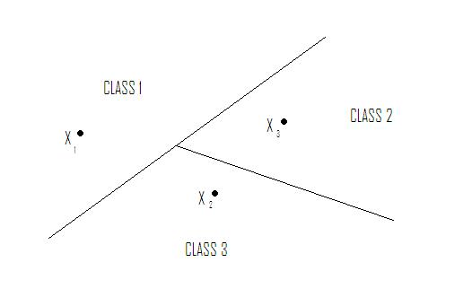
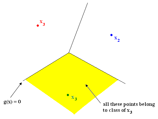
Nearest Neighbor in $ \Re ^2 $ yields tessellation (tiling of floor with 2D shapes such that 1) no holes and 2) cover all of $ \Re ^2 $ ). The tessellations separate sample space into regions. Shape of cells depends on metric chosen. See Figure 1.
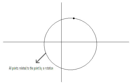
Example: if feature vectors are such that vectors related by a rotation belong to same class
$ \rightarrow $ metric should be chosen so that tiles are rotationally symmetric. See Figure 2.
Instead of working with (x,y) rotationally invariant, work with $ z=\sqrt{x^2 + y^2} $ (distance from origin)
How good is Nearest Neighbor rule?
- Training error is zero: does not measure the "goodness" of a rule
- Test error: want it to be equal to Bayes error rate, because this yields the minimum error
Nearest Neighbor error rate
Recall: Probability of error (error rate) on test data is $ P(e)=\int p(e \mid \vec{x}) p(\vec{x}) d\vec{x} $
Let $ P_d(e) $ be the error rate when d training samples are used.
Let $ P=\lim_{d \rightarrow \infty } P_{d}(e) $
Claim: limit error rate $ P=\int (1-\sum _{i=1} ^{c}p^2 (\omega _i \mid \vec{x}))p(x)dx $
Proof of claim: Given observation $ \vec{x} $, denode by $ \vec{x'}_d $ the nearest neighbor of $ \vec{x} $ among $ \{\vec{x}_1,\vec{x}_2, \cdots , \vec{x}_d \} $
$ P_d(e \mid \vec{x})=\int p_d(e \mid \vec{x}, \vec{x'}_d)p_d(\vec{x'}_d \mid \vec{x})p(x)dx $ but $ \lim _{d \rightarrow \infty } p_d (\vec{x'}_d \mid \vec{x})=\delta ({\vec{x' _d }-\vec{x}}) $
because probability that sample falls into region R centered at $ \vec{x} $ is $ P_{R}=\int _R p(\vec{x' _d})d \vec{x'}_d $.
So, if $ p(\vec{x}) \neq 0 $ (true almost everywhere), then probability that all samples fall outside R is $ \lim _{d \rightarrow \infty} {(1-P_{R})}^d =0 $
So, $ \lim _{d \rightarrow \infty} \vec{x'}_d = \vec{x} $ and $ p_d (\vec{x'}_d \mid \vec{x})=\delta (\vec{x'}_d -\vec{x})+\epsilon _d (\vec{x}) $ where $ \lim _{d \rightarrow \infty } \epsilon _d (x)=0 $
Now $ p_d (e \mid \vec{x}, \vec{x'}_d) $ = ?
Let $ \theta , \theta _1 , \theta _2 , \cdots, \theta _{d} $ be the class of $ x , x_1 , x_2 , \cdots , x_d $, respectively.
Using nearest neighbor rule, error if $ \theta \neq $class of $ \vec{x'}_d $$ =: \theta ' _d $
$ \Rightarrow p_d(e \mid \vec{x},\vec{x'}_d)=1-\sum_{i=1} ^ c p(\theta = \omega _i , \theta ' _d = \omega _i \mid \vec{x}, \vec{x'}_d ) $
$ =1- \sum _{i=1} ^c p(\omega _i \mid \vec{x}) p(\omega _i \mid \vec{x'} _d) $
Recall $ p_d (e \mid \vec{x}, \vec{x'}_d)p_d (\vec{x'}_d \mid \vec{x})d \vec{x'}_d $
You get: $ p_d (e \mid \vec{x})=(1-\sum _{i=1} ^c p(\omega _i \mid x) p(\omega _i \mid x) ) $ + {something that goes to zero as d goes to $ \infty $}
$ \lim _{d \rightarrow \infty} p_d (e \mid \vec{x})=(1- \sum _{i=1} ^c {p(\omega _i \mid x)}^2) $
Previous: Lecture 17 Next: Lecture 19


