| (29 intermediate revisions by 8 users not shown) | |||
| Line 1: | Line 1: | ||
| − | [ | + | <center><font size= 4> |
| + | '''[[ECE662]]: Statistical Pattern Recognition and Decision Making Processes''' | ||
| + | </font size> | ||
| − | [ | + | Spring 2008, [[user:mboutin|Prof. Boutin]] |
| + | [[Slectures|Slecture]] | ||
| + | <font size= 3> Collectively created by the students in [[ECE662:BoutinSpring08_OldKiwi|the class]]</font size> | ||
| + | </center> | ||
| − | + | ---- | |
| + | =Lecture 14 Lecture notes= | ||
| + | Jump to: [[ECE662_Pattern_Recognition_Decision_Making_Processes_Spring2008_sLecture_collective|Outline]]| | ||
| + | [[Lecture 1 - Introduction_OldKiwi|1]]| | ||
| + | [[Lecture 2 - Decision Hypersurfaces_OldKiwi|2]]| | ||
| + | [[Lecture 3 - Bayes classification_OldKiwi|3]]| | ||
| + | [[Lecture 4 - Bayes Classification_OldKiwi|4]]| | ||
| + | [[Lecture 5 - Discriminant Functions_OldKiwi|5]]| | ||
| + | [[Lecture 6 - Discriminant Functions_OldKiwi|6]]| | ||
| + | [[Lecture 7 - MLE and BPE_OldKiwi|7]]| | ||
| + | [[Lecture 8 - MLE, BPE and Linear Discriminant Functions_OldKiwi|8]]| | ||
| + | [[Lecture 9 - Linear Discriminant Functions_OldKiwi|9]]| | ||
| + | [[Lecture 10 - Batch Perceptron and Fisher Linear Discriminant_OldKiwi|10]]| | ||
| + | [[Lecture 11 - Fischer's Linear Discriminant again_OldKiwi|11]]| | ||
| + | [[Lecture 12 - Support Vector Machine and Quadratic Optimization Problem_OldKiwi|12]]| | ||
| + | [[Lecture 13 - Kernel function for SVMs and ANNs introduction_OldKiwi|13]]| | ||
| + | [[Lecture 14 - ANNs, Non-parametric Density Estimation (Parzen Window)_OldKiwi|14]]| | ||
| + | [[Lecture 15 - Parzen Window Method_OldKiwi|15]]| | ||
| + | [[Lecture 16 - Parzen Window Method and K-nearest Neighbor Density Estimate_OldKiwi|16]]| | ||
| + | [[Lecture 17 - Nearest Neighbors Clarification Rule and Metrics_OldKiwi|17]]| | ||
| + | [[Lecture 18 - Nearest Neighbors Clarification Rule and Metrics(Continued)_OldKiwi|18]]| | ||
| + | [[Lecture 19 - Nearest Neighbor Error Rates_OldKiwi|19]]| | ||
| + | [[Lecture 20 - Density Estimation using Series Expansion and Decision Trees_OldKiwi|20]]| | ||
| + | [[Lecture 21 - Decision Trees(Continued)_OldKiwi|21]]| | ||
| + | [[Lecture 22 - Decision Trees and Clustering_OldKiwi|22]]| | ||
| + | [[Lecture 23 - Spanning Trees_OldKiwi|23]]| | ||
| + | [[Lecture 24 - Clustering and Hierarchical Clustering_OldKiwi|24]]| | ||
| + | [[Lecture 25 - Clustering Algorithms_OldKiwi|25]]| | ||
| + | [[Lecture 26 - Statistical Clustering Methods_OldKiwi|26]]| | ||
| + | [[Lecture 27 - Clustering by finding valleys of densities_OldKiwi|27]]| | ||
| + | [[Lecture 28 - Final lecture_OldKiwi|28]] | ||
| + | ---- | ||
| + | ---- | ||
| + | ==Artificial Neural Networks== | ||
| + | (Continued from [[Lecture 13 - Kernel function for SVMs and ANNs introduction_OldKiwi|Lecture 13]]) | ||
| − | + | [[Image:ANN_OldKiwi.gif]] | |
| − | Samples | + | Samples |
| − | + | <math> x_1 , \cdots , x_d </math> | |
| − | + | ||
| − | |||
| − | |||
<math> J(\vec{w}) = \displaystyle \sum _{l=1} ^{d} \frac{||\vec{t}_l - \vec{z}_l ||^2} {2}</math> | <math> J(\vec{w}) = \displaystyle \sum _{l=1} ^{d} \frac{||\vec{t}_l - \vec{z}_l ||^2} {2}</math> | ||
| − | Use | + | Use gradient descent |
<math>\vec{w} (n+1)= \vec{w}(n) - \eta (n) \left( \frac{\partial J}{\partial w_1}, \cdots , \frac{\partial J }{\partial w_{last}}\right)</math> | <math>\vec{w} (n+1)= \vec{w}(n) - \eta (n) \left( \frac{\partial J}{\partial w_1}, \cdots , \frac{\partial J }{\partial w_{last}}\right)</math> | ||
for simplicity, assume d=1 | for simplicity, assume d=1 | ||
| − | To compute <math> \frac{\partial J}{\partial w_i}</math>, use chain rule. | + | To compute <math> \frac{\partial J}{\partial w_i}</math>, use the chain rule. |
| Line 37: | Line 73: | ||
<math> \quad \qquad = -(t_{k0}-z_{k0})f' \left(\displaystyle \sum _{j \rightarrow k_0} w_{jk_0}y_{j} \right) y_{j0}</math> | <math> \quad \qquad = -(t_{k0}-z_{k0})f' \left(\displaystyle \sum _{j \rightarrow k_0} w_{jk_0}y_{j} \right) y_{j0}</math> | ||
| − | + | [[Image:pic1_OldKiwi.jpg]] | |
| Line 46: | Line 82: | ||
<math> \quad \qquad = w_{jk} (n) + \eta (n) (t_k -z_k) f' \left( \displaystyle \sum _{j \rightarrow k} w_{jk}y_j \right) y_j | <math> \quad \qquad = w_{jk} (n) + \eta (n) (t_k -z_k) f' \left( \displaystyle \sum _{j \rightarrow k} w_{jk}y_j \right) y_j | ||
</math> | </math> | ||
| − | For "input units to hidden units" weights | + | |
| − | <math> w_{ij} </math> | + | For "input units to hidden units" weights <math>w_{ij}</math>, pick <math>i_{0},j_{0}</math> |
| − | <math>i_{0},j_{0}</math> | + | |
<math> \displaystyle \frac{\partial J}{\partial w_{i_0 j_0}}=\displaystyle \frac{\partial J}{\partial y_{j_0}} \cdot \displaystyle \frac{\partial y_{j_0}}{\partial \displaystyle \sum _{i \rightarrow j_0} w_{i j_0} x_{i}} \cdot \displaystyle \frac{\partial \displaystyle \sum _{i \rightarrow j_0} w_{ij_0 } x_{i}} {\partial w_{i_0 j_0}}</math> | <math> \displaystyle \frac{\partial J}{\partial w_{i_0 j_0}}=\displaystyle \frac{\partial J}{\partial y_{j_0}} \cdot \displaystyle \frac{\partial y_{j_0}}{\partial \displaystyle \sum _{i \rightarrow j_0} w_{i j_0} x_{i}} \cdot \displaystyle \frac{\partial \displaystyle \sum _{i \rightarrow j_0} w_{ij_0 } x_{i}} {\partial w_{i_0 j_0}}</math> | ||
| Line 54: | Line 89: | ||
</math> | </math> | ||
| − | <math> \quad \qquad = \displaystyle \ | + | <math>\quad \qquad = \displaystyle \sum_{k=1}^{c}\frac{\partial J}{\partial z_k} \cdot \frac{\partial z_k}{\partial y_{j0}} \cdot f'_{j0} \left(\displaystyle \sum _{i \rightarrow j_0} w_{j0} x_i \right) x_{i0}</math> |
| − | <math> \quad \qquad = - \displaystyle \sum _{k=1} ^{c} (t_k - z_k) f'_{k} \cdot f'_{j0} \cdot x_{ | + | <math> \quad \qquad = - \displaystyle \sum _{k=1} ^{c} (t_k - z_k) {f'}_{k} \cdot {f'}_{j0} \cdot x_{i_0} </math> |
| − | </math> | + | |
| + | [[Image:lec14_pic2_OldKiwi.jpg]] | ||
| − | |||
=> update rule for weights between input units to hidden units. | => update rule for weights between input units to hidden units. | ||
| Line 68: | Line 103: | ||
| − | + | ==Non-Parametric Density Estimation== | |
| − | + | ||
| − | + | ||
| − | + | ||
| − | + | ||
| − | + | ||
| − | + | ||
| − | + | ||
| − | + | ||
| − | + | ||
| − | + | ||
| − | + | ||
| − | + | ||
| − | + | ||
| − | + | ||
It is not a very accurate estimate of the density but we are more concerned with making the right decisions rather than estimating the density correctly. | It is not a very accurate estimate of the density but we are more concerned with making the right decisions rather than estimating the density correctly. | ||
| Line 109: | Line 130: | ||
<math> {R}^{n}</math> | <math> {R}^{n}</math> | ||
| − | + | [[Image:Example1_OldKiwi.jpg]] | |
For the sake of simplicity we can divide the region into cubes with side length h. | For the sake of simplicity we can divide the region into cubes with side length h. | ||
| − | + | [[Image:Jc_npm_OldKiwi.gif]] | |
Count how many samples fall into that region R | Count how many samples fall into that region R | ||
| Line 149: | Line 170: | ||
Once again the problem is if we fix #of samples and let vol(R) ->0 then for most region #of samples =0! sp p(x0)=0! | Once again the problem is if we fix #of samples and let vol(R) ->0 then for most region #of samples =0! sp p(x0)=0! | ||
| − | So in 1-D we get a estimate which looks like spikes | + | So in 1-D we get a estimate which looks like spikes. |
| Line 182: | Line 203: | ||
Techniques to build such sequences: | Techniques to build such sequences: | ||
| − | + | ==Parzen Window Method== | |
pick Ri such that Vi= <math> 1/\sqrt{i}</math> | pick Ri such that Vi= <math> 1/\sqrt{i}</math> | ||
| Line 192: | Line 213: | ||
Parzen windows can be regarded as a generalization of k-nearest neighbor techniques. Rather than choosing the k nearest neighbors of a test point and labelling the test point with the weighted majority of its neighbors' votes, one can consider all points in the voting scheme and assign their weight by means of the kernel function. With Gaussian kernels, the weight decreases exponentially with the square of the distance, so far away points are practically irrelevant. The width $\sigma$ of the Guassian determines the relative weighting of near and far points. Tuning this parameter controls the predictive power of the system. We have empirically optimized the value. | Parzen windows can be regarded as a generalization of k-nearest neighbor techniques. Rather than choosing the k nearest neighbors of a test point and labelling the test point with the weighted majority of its neighbors' votes, one can consider all points in the voting scheme and assign their weight by means of the kernel function. With Gaussian kernels, the weight decreases exponentially with the square of the distance, so far away points are practically irrelevant. The width $\sigma$ of the Guassian determines the relative weighting of near and far points. Tuning this parameter controls the predictive power of the system. We have empirically optimized the value. | ||
| − | + | ===Examples of Parzen Windows=== | |
The parzen window is defined by |parzen_window| | The parzen window is defined by |parzen_window| | ||
| Line 207: | Line 228: | ||
d is chosen to be 2. | d is chosen to be 2. | ||
| − | + | [[Image:Example3_OldKiwi.jpg|frame|center|Two dimensional circularly symmetric normal Parzen Window]] | |
| + | [[Image:Example4_OldKiwi.jpg|frame|center|Two dimensional square Parzan Window]] | ||
| − | + | ==K-Nearest Neighbors Method== | |
| − | + | ||
| − | + | ||
| − | + | ||
| − | + | ||
| − | + | ||
| − | + | ||
Pick Ri so that Ki= <math> \sqrt{i} </math> | Pick Ri so that Ki= <math> \sqrt{i} </math> | ||
| Line 227: | Line 243: | ||
| − | + | ==Visual Comparison (for Parzen Windows):== | |
| + | [[Image:Example6_OldKiwi.jpg]] | ||
| + | [[Image:Example7_OldKiwi.jpg]] | ||
| − | + | ==Visual Comparions between Parzen Winows & K-Nearest Neighbor:== | |
| − | + | ||
| + | [[Image:Example8_OldKiwi.jpg]] | ||
| − | |||
| − | |||
| + | ==Parametric v.s. Nonparametric Methods== | ||
| − | + | [[Parametric Model_OldKiwi|Parametric Model]] & [[Non-parametric Model_OldKiwi|Non-parametric Model]] | |
| − | + | ||
| − | + | ||
| − | [[Parametric Model_OldKiwi]] & [[Non-parametric Model_OldKiwi]] | + | |
It's worth to note that it's not one hundred percent right when we say that non-parametric methods are "model-free" or free of distribution assumptions. Take nearest neighbor for example, some kind of distance measure has to be used to identifying the "nearest" neighbor. Although the method didn't assume a specific distribution, the distance measure is distribution-related in some sense. (Euclidean and Mahalanobis distances are closely related to multivariate Gaussian distribution.) Compared to parametric methods, non-parametric ones only "vaguely" or "remotely" related to specific distributions and, therefore, are a lot flexible and less sensitive to violation of distribution assumptions. | It's worth to note that it's not one hundred percent right when we say that non-parametric methods are "model-free" or free of distribution assumptions. Take nearest neighbor for example, some kind of distance measure has to be used to identifying the "nearest" neighbor. Although the method didn't assume a specific distribution, the distance measure is distribution-related in some sense. (Euclidean and Mahalanobis distances are closely related to multivariate Gaussian distribution.) Compared to parametric methods, non-parametric ones only "vaguely" or "remotely" related to specific distributions and, therefore, are a lot flexible and less sensitive to violation of distribution assumptions. | ||
| Line 248: | Line 262: | ||
| − | + | ==Advantages of Non-parametric Estimation Methods== | |
* Same procedure can be used for unimodal normal and bimodal mixture. | * Same procedure can be used for unimodal normal and bimodal mixture. | ||
* We do not need to make assumption about the distribution ahead of time. | * We do not need to make assumption about the distribution ahead of time. | ||
| Line 254: | Line 268: | ||
| − | + | ==Disadvantages of Non-parametric Estimation Methods== | |
* The cardinality of the sample set should be very large (much larger than the cardinality when the form of density is known) . | * The cardinality of the sample set should be very large (much larger than the cardinality when the form of density is known) . | ||
* Very high computation time and huge storage required. | * Very high computation time and huge storage required. | ||
| Line 260: | Line 274: | ||
* These methods are very sensitive to the choice of the window size (If too small, most of the volume will be empty, and the estimate will be erratic, if too large: important variations may be lost due to averaging.) | * These methods are very sensitive to the choice of the window size (If too small, most of the volume will be empty, and the estimate will be erratic, if too large: important variations may be lost due to averaging.) | ||
* It may be the case that a cell volume appropriate for one region of the feature space might be entirely unsuitable in a different region. | * It may be the case that a cell volume appropriate for one region of the feature space might be entirely unsuitable in a different region. | ||
| + | ---- | ||
| + | Previous: [[Lecture_13_-_Kernel_function_for_SVMs_and_ANNs_introduction_OldKiwi|Lecture 13]] | ||
| + | Next: [[Lecture_15_-_Parzen_Window_Method_OldKiwi|Lecture 15]] | ||
| − | + | [[ECE662:BoutinSpring08_OldKiwi|Back to ECE662 Spring 2008 Prof. Boutin]] | |
| − | + | [[Category:ECE662]] | |
| − | [ | + | [[Category:decision theory]] |
| − | + | [[Category:lecture notes]] | |
| − | + | [[Category:pattern recognition]] | |
| − | + | [[Category:slecture]] | |
| − | + | ||
| − | + | ||
| − | + | ||
| − | + | ||
| − | + | ||
| − | + | ||
| − | + | ||
| − | + | ||
| − | + | ||
| − | + | ||
| − | + | ||
| − | + | ||
| − | + | ||
| − | + | ||
| − | [ | + | |
Latest revision as of 11:21, 10 June 2013
ECE662: Statistical Pattern Recognition and Decision Making Processes
Spring 2008, Prof. Boutin
Collectively created by the students in the class
Contents
- 1 Lecture 14 Lecture notes
- 1.1 Artificial Neural Networks
- 1.2 Non-Parametric Density Estimation
- 1.3 Parzen Window Method
- 1.4 K-Nearest Neighbors Method
- 1.5 Visual Comparison (for Parzen Windows):
- 1.6 Visual Comparions between Parzen Winows & K-Nearest Neighbor:
- 1.7 Parametric v.s. Nonparametric Methods
- 1.8 Advantages of Non-parametric Estimation Methods
- 1.9 Disadvantages of Non-parametric Estimation Methods
Lecture 14 Lecture notes
Jump to: Outline| 1| 2| 3| 4| 5| 6| 7| 8| 9| 10| 11| 12| 13| 14| 15| 16| 17| 18| 19| 20| 21| 22| 23| 24| 25| 26| 27| 28
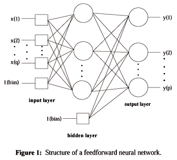
Artificial Neural Networks
(Continued from Lecture 13)
Samples
$ x_1 , \cdots , x_d $
$ J(\vec{w}) = \displaystyle \sum _{l=1} ^{d} \frac{||\vec{t}_l - \vec{z}_l ||^2} {2} $
Use gradient descent
$ \vec{w} (n+1)= \vec{w}(n) - \eta (n) \left( \frac{\partial J}{\partial w_1}, \cdots , \frac{\partial J }{\partial w_{last}}\right) $
for simplicity, assume d=1 To compute $ \frac{\partial J}{\partial w_i} $, use the chain rule.
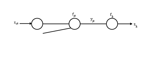
For "hidden units to output units" weights $ w_{jk} $, pick $ j_{0}, k_{0} $
$ \displaystyle \frac{\partial J}{\partial w_{j_0 k_0}}=\displaystyle \frac{\partial J}{\partial z_{k_0}} \cdot \displaystyle \frac{\partial z_{k_0}}{\partial \displaystyle \sum _{j \rightarrow k_0} w_{j_0 k_0} y_{j}} \cdot \displaystyle \frac{\partial \displaystyle \sum _{j \rightarrow k_0} w_{j_0 k_0} y_{j}} {\partial w_{j_0 k_0}} $
$ \quad \qquad = \displaystyle \frac{\displaystyle \sum_{k} \frac{1}{2}(t_k - z_k)^2}{\partial z_{k_0}} f' \left( \displaystyle \sum_{j \rightarrow k_{0}} w_{jk_0}y_{j} \right) y_{j0} $
$ \quad \qquad = -(t_{k0}-z_{k0})f' \left(\displaystyle \sum _{j \rightarrow k_0} w_{jk_0}y_{j} \right) y_{j0} $
=> Update rule for weights between hidden units and output units
$ w_{jk}(n+1)=w_{jk}(n)- \eta (n) \frac{\partial J}{\partial w_{jk}} $
$ \quad \qquad = w_{jk} (n) + \eta (n) (t_k -z_k) f' \left( \displaystyle \sum _{j \rightarrow k} w_{jk}y_j \right) y_j $
For "input units to hidden units" weights $ w_{ij} $, pick $ i_{0},j_{0} $
$ \displaystyle \frac{\partial J}{\partial w_{i_0 j_0}}=\displaystyle \frac{\partial J}{\partial y_{j_0}} \cdot \displaystyle \frac{\partial y_{j_0}}{\partial \displaystyle \sum _{i \rightarrow j_0} w_{i j_0} x_{i}} \cdot \displaystyle \frac{\partial \displaystyle \sum _{i \rightarrow j_0} w_{ij_0 } x_{i}} {\partial w_{i_0 j_0}} $ $ \quad \qquad = \displaystyle \frac{\partial J}{\partial y_{j0}} f'_{j0} \left( \displaystyle \sum _{i \rightarrow j_0} w_{j0} x_i \right) x_{i0} $
$ \quad \qquad = \displaystyle \sum_{k=1}^{c}\frac{\partial J}{\partial z_k} \cdot \frac{\partial z_k}{\partial y_{j0}} \cdot f'_{j0} \left(\displaystyle \sum _{i \rightarrow j_0} w_{j0} x_i \right) x_{i0} $
$ \quad \qquad = - \displaystyle \sum _{k=1} ^{c} (t_k - z_k) {f'}_{k} \cdot {f'}_{j0} \cdot x_{i_0} $
=> update rule for weights between input units to hidden units.
$ w_{ij}(n+1)=w_{ij}(n)- \eta (n) \frac{\partial J}{\partial w_{ij}} $
$ \quad \qquad = w_{jk}(n)+ \eta (n) \displaystyle \sum _k (t_k -z_k) f'_k \left( \displaystyle \sum _{j \rightarrow k} w_{jk} y_k \right) w_{jk} f'_j (\displaystyle \sum _{i \rightarrow j} w_{ij} x_i) x_i $
Non-Parametric Density Estimation
It is not a very accurate estimate of the density but we are more concerned with making the right decisions rather than estimating the density correctly.
We rely on the fact that
P=Probability{x belongs to R}
R is a region of feature space
$ \quad P=\int p(X)dX $
To estimate P :
$ \quad P=\int p(X)dX = p(x0)vol(R) $
if p(X) is continuous near xo and and R is small
The Idea behind this method is:
Draw samples at random X1,X2,....Xd
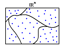
Divide the feature space into regions in |khh20|
$ {R}^{n} $
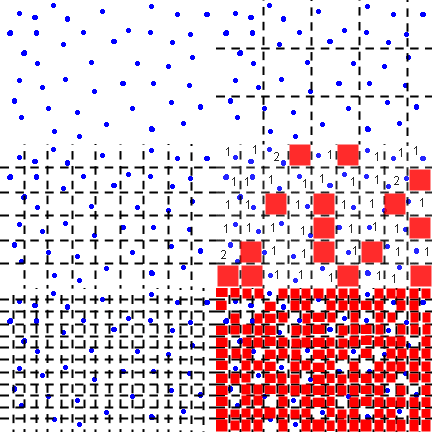
For the sake of simplicity we can divide the region into cubes with side length h.
Count how many samples fall into that region R
P=Prob(X is in R) = #of samples in R/d where d is total number of samples
But
$ \quad P=\int p(X)dX = p(x0)vol(R) $
so
p(x0) vol(R) = #of samples in R / d
so
p(x0)=#of samples in R/(d*vol(R))
To make $ \hat{p(x0)} $ converge to p(x0) we should
1) Fix the volume R and take a large number of samples
then #of samples in R/d goes to P
so goes to P/vol(R)
Problem : P/vol(R) is not p(x0)!
So we should also
2) Let vol(R) go to zero
Once again the problem is if we fix #of samples and let vol(R) ->0 then for most region #of samples =0! sp p(x0)=0!
So in 1-D we get a estimate which looks like spikes.
Consider a sequence of regions containing $ \vec{x0} $
{Ri}i belongs to N , x0 belongs to Ri for all i
and an infinite sequence of samples
X1,X2,.....={Xk} k is in the N
Construct set of samples Si={X1,X2.....Xi}
Pi=Probability that |khh23|
$ \vec{x} \epsilon Ri $
Vi=Volume of Ri
Ki=#of samples from Si falling in Ri
pi=Ki/(i*Vi)
1) $ \lim_{i\rightarrow inf}=0 This ensures Pi/Vi converges to p(x0) $ 2) $ \lim_{i\rightarrow inf} Ki =inf $
3) $ \lim_{i\rightarrow inf} Ki/i =0 $
Techniques to build such sequences:
Parzen Window Method
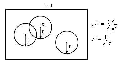
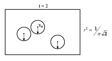
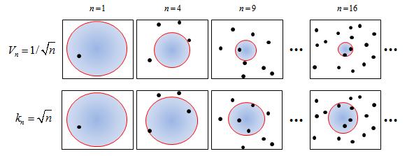
pick Ri such that Vi= $ 1/\sqrt{i} $
Parzen windows classification is a technique for nonparametric density estimation, which can also be used for classification. Using a given kernel function, the technique approximates a given training set distribution via a linear combination of kernels centered on the observed points. In this work, we separately approximate densities for each of the two classes, and we assign a test point to the class with maximal posterior probability.
The resulting algorithm is extremely simple and closely related to support vector machines. The Parzen windows classification algorithm does not require any training phase; however, the lack of sparseness makes the test phase quite slow. Furthermore, although asymptotical convergence guarantees on the perfomance of Parzen windows classifiers exist, no such guarantees exist for finite sample sizes.
Parzen windows can be regarded as a generalization of k-nearest neighbor techniques. Rather than choosing the k nearest neighbors of a test point and labelling the test point with the weighted majority of its neighbors' votes, one can consider all points in the voting scheme and assign their weight by means of the kernel function. With Gaussian kernels, the weight decreases exponentially with the square of the distance, so far away points are practically irrelevant. The width $\sigma$ of the Guassian determines the relative weighting of near and far points. Tuning this parameter controls the predictive power of the system. We have empirically optimized the value.
Examples of Parzen Windows
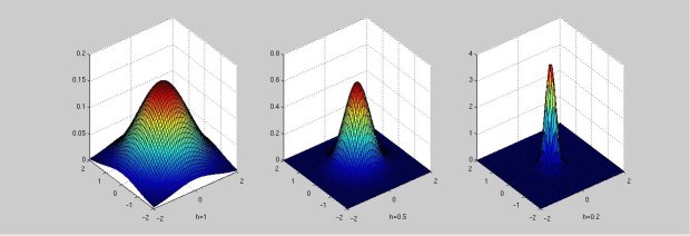
The parzen window is defined by |parzen_window| $ \delta\left(\mathbf{x}\right)=\frac{1}{V}\varphi\left(\frac{\mathbf{x}}{h}\right) $
where |V|
$ V=h^d $
d is the number of dimensions.
The values of 'h' parameter are chosen to be 1, 0.5 and 0.2.
d is chosen to be 2.
K-Nearest Neighbors Method
Pick Ri so that Ki= $ \sqrt{i} $
The k-nearest neighbor algorithm is amongst the simplest of all machine learning algorithms. An object is classified by a majority vote of its neighbors, with the object being assigned to the class most common amongst its k nearest neighbors. k is a positive integer, typically small. If k = 1, then the object is simply assigned to the class of its nearest neighbor. In binary (two class) classification problems, it is helpful to choose k to be an odd number as this avoids tied votes.
The naive version of the algorithm is easy to implement by computing the distances from the test sample to all stored vectors, but it is computationally intensive, especially when the size of the training set grows. Many nearest neighbor search algorithms have been proposed over the years; these generally seek to reduce the number of distance evaluations actually performed. The nearest neighbor algorithm has some strong consistency results. As the amount of data approaches infinity, the algorithm is guaranteed to yield an error rate no worse than twice the Bayes error rate (the minimum achievable error rate given the distribution of the data). k-nearest neighbor is guaranteed to approach the Bayes error rate, for some value of k (where k increases as a function of the number of data points).
Here is a link to a k-Nearest Neighbor demo using a Java applet: http://www.cs.cmu.edu/~zhuxj/courseproject/knndemo/KNN.html
Visual Comparison (for Parzen Windows):
Visual Comparions between Parzen Winows & K-Nearest Neighbor:
Parametric v.s. Nonparametric Methods
Parametric Model & Non-parametric Model
It's worth to note that it's not one hundred percent right when we say that non-parametric methods are "model-free" or free of distribution assumptions. Take nearest neighbor for example, some kind of distance measure has to be used to identifying the "nearest" neighbor. Although the method didn't assume a specific distribution, the distance measure is distribution-related in some sense. (Euclidean and Mahalanobis distances are closely related to multivariate Gaussian distribution.) Compared to parametric methods, non-parametric ones only "vaguely" or "remotely" related to specific distributions and, therefore, are a lot flexible and less sensitive to violation of distribution assumptions.
Another characteristic found to be helpful in discriminating the two is that: the number of parameters in parametric models is fixed a priori and independent of the size of the dataset, while the number of statistics used for non-parametric models are usually dependent on the size of the dataset (e.g. more statistics for larger datasets)
Advantages of Non-parametric Estimation Methods
- Same procedure can be used for unimodal normal and bimodal mixture.
- We do not need to make assumption about the distribution ahead of time.
- With enough samples, we are assured of convergence to an arbitrarily complicated target density
Disadvantages of Non-parametric Estimation Methods
- The cardinality of the sample set should be very large (much larger than the cardinality when the form of density is known) .
- Very high computation time and huge storage required.
- Curse of dimensionality (see [Curse of Dimensionality])
- These methods are very sensitive to the choice of the window size (If too small, most of the volume will be empty, and the estimate will be erratic, if too large: important variations may be lost due to averaging.)
- It may be the case that a cell volume appropriate for one region of the feature space might be entirely unsuitable in a different region.
Previous: Lecture 13 Next: Lecture 15

