(→Algorithms for clustering from feature vector) |
|||
| (25 intermediate revisions by 8 users not shown) | |||
| Line 1: | Line 1: | ||
| − | = | + | <center><font size= 4> |
| + | '''[[ECE662]]: Statistical Pattern Recognition and Decision Making Processes''' | ||
| + | </font size> | ||
| + | Spring 2008, [[user:mboutin|Prof. Boutin]] | ||
| + | [[Slectures|Slecture]] | ||
| + | <font size= 3> Collectively created by the students in [[ECE662:BoutinSpring08_OldKiwi|the class]]</font size> | ||
| + | </center> | ||
| − | == | + | ---- |
| + | =Lecture 25 Lecture notes= | ||
| + | Jump to: [[ECE662_Pattern_Recognition_Decision_Making_Processes_Spring2008_sLecture_collective|Outline]]| | ||
| + | [[Lecture 1 - Introduction_OldKiwi|1]]| | ||
| + | [[Lecture 2 - Decision Hypersurfaces_OldKiwi|2]]| | ||
| + | [[Lecture 3 - Bayes classification_OldKiwi|3]]| | ||
| + | [[Lecture 4 - Bayes Classification_OldKiwi|4]]| | ||
| + | [[Lecture 5 - Discriminant Functions_OldKiwi|5]]| | ||
| + | [[Lecture 6 - Discriminant Functions_OldKiwi|6]]| | ||
| + | [[Lecture 7 - MLE and BPE_OldKiwi|7]]| | ||
| + | [[Lecture 8 - MLE, BPE and Linear Discriminant Functions_OldKiwi|8]]| | ||
| + | [[Lecture 9 - Linear Discriminant Functions_OldKiwi|9]]| | ||
| + | [[Lecture 10 - Batch Perceptron and Fisher Linear Discriminant_OldKiwi|10]]| | ||
| + | [[Lecture 11 - Fischer's Linear Discriminant again_OldKiwi|11]]| | ||
| + | [[Lecture 12 - Support Vector Machine and Quadratic Optimization Problem_OldKiwi|12]]| | ||
| + | [[Lecture 13 - Kernel function for SVMs and ANNs introduction_OldKiwi|13]]| | ||
| + | [[Lecture 14 - ANNs, Non-parametric Density Estimation (Parzen Window)_OldKiwi|14]]| | ||
| + | [[Lecture 15 - Parzen Window Method_OldKiwi|15]]| | ||
| + | [[Lecture 16 - Parzen Window Method and K-nearest Neighbor Density Estimate_OldKiwi|16]]| | ||
| + | [[Lecture 17 - Nearest Neighbors Clarification Rule and Metrics_OldKiwi|17]]| | ||
| + | [[Lecture 18 - Nearest Neighbors Clarification Rule and Metrics(Continued)_OldKiwi|18]]| | ||
| + | [[Lecture 19 - Nearest Neighbor Error Rates_OldKiwi|19]]| | ||
| + | [[Lecture 20 - Density Estimation using Series Expansion and Decision Trees_OldKiwi|20]]| | ||
| + | [[Lecture 21 - Decision Trees(Continued)_OldKiwi|21]]| | ||
| + | [[Lecture 22 - Decision Trees and Clustering_OldKiwi|22]]| | ||
| + | [[Lecture 23 - Spanning Trees_OldKiwi|23]]| | ||
| + | [[Lecture 24 - Clustering and Hierarchical Clustering_OldKiwi|24]]| | ||
| + | [[Lecture 25 - Clustering Algorithms_OldKiwi|25]]| | ||
| + | [[Lecture 26 - Statistical Clustering Methods_OldKiwi|26]]| | ||
| + | [[Lecture 27 - Clustering by finding valleys of densities_OldKiwi|27]]| | ||
| + | [[Lecture 28 - Final lecture_OldKiwi|28]] | ||
| + | ---- | ||
| + | ---- | ||
| + | == Clustering Methods - A summary == | ||
| − | + | [[Image:summary_Clustering_methods_OldKiwi.jpg|frame|center|Figure 1]] | |
| + | Ward's method is supposedly the best. What this means is when there are natural clusters in the dataset, then almost all of above mentioned methods work well, but of them Ward's method works the best. | ||
| + | |||
| + | But these methods have a serious shortcoming. They tend to find compact clusters because they depend on distances between data points. | ||
| + | |||
| + | *Illustrating figure can be inserted | ||
| + | |||
| + | So, if the natural clustering in data points is elongated and interspersed, these methods may break one elongated cluster into many, and may mix different elongated clusters into one. So, we need feature vectors to find natural clusters, if they are of arbitrary shape and contain arbitrary number of points. | ||
| + | |||
| + | In a high dimension feature space, data points are never adequate. The space is always sparse, and typically distance between any two data points is of the same order. So, the approach used is to project data onto lower dimensions. It doesn't matter which features or combination of features are used to project, because the objective is to have a indexing mechanism for the database. | ||
| + | |||
| + | [[Image:Lec25_proj_clusters_OldKiwi.PNG|frame|center|Figure 3]] | ||
| + | |||
| + | == Algorithms for clustering from feature vector == | ||
| + | |||
| + | Called "Partitional clustering" in Jain and Dude as opposed to "hierarchical clustering" | ||
Clustering feature vectors = finding separation between clusters but these are not known | Clustering feature vectors = finding separation between clusters but these are not known | ||
| + | |||
| + | Note: "Partitional Clustering" is advantageous in the sense that it provides a set of partition rules that can be generalized to future unseen data. For clustering methods based on pair-wise distance, such rules are not always available. | ||
| + | |||
| + | [[Image:Lec25_clusters_fv_OldKiwi.PNG|frame|center|Figure 4]] | ||
<<Picture>> | <<Picture>> | ||
| Line 27: | Line 85: | ||
<math>S_w= \sum _{i=1, X_i \in S_1} ^d ||X_i - \mu _1||^2 + \sum _{i=1, X_i \in S_2} ^d ||X_i - \mu _2||^2</math> (2-1) | <math>S_w= \sum _{i=1, X_i \in S_1} ^d ||X_i - \mu _1||^2 + \sum _{i=1, X_i \in S_2} ^d ||X_i - \mu _2||^2</math> (2-1) | ||
| − | <math>\mu _1 = \frac{1}{|S_1|} \ | + | <math>\mu _1 = \frac{1}{|S_1|} \sum _{X_i \in S_1} X_i</math>, <math>\mu _2 = \frac{1}{|S_2|} \sum _{X_i \in S_2} X_i</math> (2-2) |
<math>S_m</math> is "mixture scatter matrix" | <math>S_m</math> is "mixture scatter matrix" | ||
| Line 93: | Line 151: | ||
Look at evolution of J for c increase (similarity scale) | Look at evolution of J for c increase (similarity scale) | ||
| + | |||
| + | [[Image:Lec25_nat_clusters_J_OldKiwi.PNG|frame|center|Figure 5]] | ||
| + | |||
| + | An important J | ||
| + | |||
| + | "Square error criterion" | ||
| + | |||
| + | <math>J=\sum _{j=1} ^{c} \sum _{X_i \in S_j}||X_i - \mu _ j||^2</math> (2-8) | ||
| + | |||
| + | where <math>\mu _j = \frac{1}{|S_j|} \sum _{X_i \in S_j} X_i</math> (2-9) | ||
| + | |||
| + | * Good when clusters are compact, well separated | ||
| + | * Sensitive to outliers | ||
| + | |||
| + | [[Image:Lec25_J_criterion_OldKiwi.PNG|frame|center|Figure 6]] | ||
| + | |||
| + | <math>J=\sum _{j=1} ^{c} \sum _{X_i \in S_j} ||X_i - \mu_j||_{L1}</math> is more robust to outliers | ||
| + | |||
| + | Can use other types of similarity measure | ||
| + | |||
| + | <math>S(X_1, X_2)=\frac{X_1 \cdot X_2}{||X_1||||X_2||}</math> (2-10) | ||
| + | |||
| + | to speed up optimization of J | ||
| + | |||
| + | Use "Nearest mean reclassification rule" | ||
| + | |||
| + | * choose initial partition <math>S_1, S_2 , \cdots , S_c</math> (2-11) | ||
| + | |||
| + | * calculate <math>\mu _1 , \mu _2 , \cdots , \mu _c </math> | ||
| + | |||
| + | * reclsssify each <math>X_i</math> to the class of the nearest mean | ||
| + | |||
| + | * If cluster have changed, repeat | ||
| + | |||
| + | Note: <math>X_i</math> class of its nearest mean | ||
| + | |||
| + | is same as choosing the move for <math>X_i</math> that moves <math>\Delta J</math> as negative as possible | ||
| + | because <math>J=\sum _{j=1} ^{c} \sum _{X_i \in S_j} ||X_i - \mu _j||^2</math> (2-12) | ||
| + | |||
| + | If <math>X_{io} \in S_{jo} \rightarrow X_{io} \in S_{\bar{j0}}</math>, | ||
| + | |||
| + | <math>J \Rightarrow \sum _{j=1} ^{c} \sum _{X_i \in S_j} ||X_i - \mu_j||^2 - ||X_{io}-\mu _{jo}||^2 + ||X_{io} - \mu _{\bar {jo}}||^2</math> (2-13) | ||
| + | |||
| + | <math>\Delta J</math> is as negative as possible when <math>||X_{io} - \mu _{\bar {jo}}||^2</math> is <math>\begin{smallmatrix} | ||
| + | min\\ | ||
| + | j | ||
| + | \end{smallmatrix} ||X_i -\mu _j||^2</math> (2-14) | ||
| + | |||
| + | Can use FORGY, CLUSTER | ||
| + | |||
| + | Observation | ||
| + | |||
| + | <math>J= \cdots = \sum _{j=1} ^c \frac{1}{|S_j|} \sum _{X_i \in S_j , X_k \in S_j} \frac{||X_i-X_k||^2}{2}</math> (2-15) | ||
| + | |||
| + | This is a distance based clustering method. | ||
| + | |||
| + | No need for feature vector | ||
| + | ---- | ||
| + | Previous: [[Lecture_24_-_Clustering_and_Hierarchical_Clustering_Old_Kiwi|Lecture 24]] | ||
| + | Next: [[Lecture_26_-_Statistical_Clustering_Methods_Old_Kiwi|Lecture 26]] | ||
| + | |||
| + | |||
| + | [[ECE662:BoutinSpring08_OldKiwi|Back to ECE662 Spring 2008 Prof. Boutin]] | ||
| + | [[Category:ECE662]] | ||
| + | [[Category:decision theory]] | ||
| + | [[Category:lecture notes]] | ||
| + | [[Category:pattern recognition]] | ||
| + | [[Category:slecture]] | ||
Latest revision as of 11:24, 10 June 2013
ECE662: Statistical Pattern Recognition and Decision Making Processes
Spring 2008, Prof. Boutin
Collectively created by the students in the class
Lecture 25 Lecture notes
Jump to: Outline| 1| 2| 3| 4| 5| 6| 7| 8| 9| 10| 11| 12| 13| 14| 15| 16| 17| 18| 19| 20| 21| 22| 23| 24| 25| 26| 27| 28
Clustering Methods - A summary
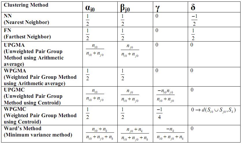
Ward's method is supposedly the best. What this means is when there are natural clusters in the dataset, then almost all of above mentioned methods work well, but of them Ward's method works the best.
But these methods have a serious shortcoming. They tend to find compact clusters because they depend on distances between data points.
- Illustrating figure can be inserted
So, if the natural clustering in data points is elongated and interspersed, these methods may break one elongated cluster into many, and may mix different elongated clusters into one. So, we need feature vectors to find natural clusters, if they are of arbitrary shape and contain arbitrary number of points.
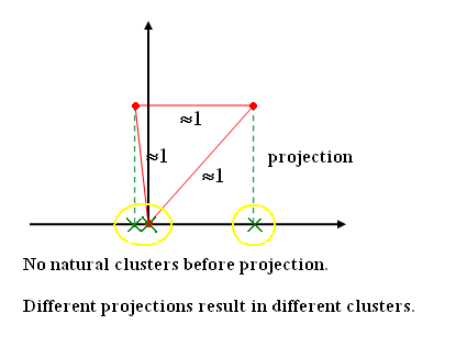
In a high dimension feature space, data points are never adequate. The space is always sparse, and typically distance between any two data points is of the same order. So, the approach used is to project data onto lower dimensions. It doesn't matter which features or combination of features are used to project, because the objective is to have a indexing mechanism for the database.
Algorithms for clustering from feature vector
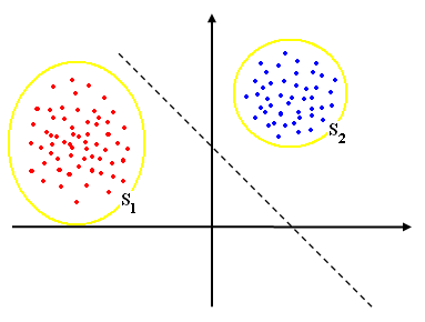
Called "Partitional clustering" in Jain and Dude as opposed to "hierarchical clustering" Clustering feature vectors = finding separation between clusters but these are not known
Note: "Partitional Clustering" is advantageous in the sense that it provides a set of partition rules that can be generalized to future unseen data. For clustering methods based on pair-wise distance, such rules are not always available.
<<Picture>>
We have a set of points S Want to find subsets $ S_1 , S_2 , \cdots , S_c $ such that $ S=S_1 \cup S_2 \cup \cdots \cup S_c $ and $ S_i \cap S_j = \phi $
need to define "clustering criteria" i.e., a measure of how natural the clustering is.
if c=2,
consider
$ J=tr(S_m ^{-1} S_w) $
where $ S_w $ is "within class scatter matrix"
$ S_w= \sum _{i=1, X_i \in S_1} ^d ||X_i - \mu _1||^2 + \sum _{i=1, X_i \in S_2} ^d ||X_i - \mu _2||^2 $ (2-1)
$ \mu _1 = \frac{1}{|S_1|} \sum _{X_i \in S_1} X_i $, $ \mu _2 = \frac{1}{|S_2|} \sum _{X_i \in S_2} X_i $ (2-2)
$ S_m $ is "mixture scatter matrix"
$ S_m= \sum _{i=1} ^d ||X_i - \mu||^2 $, $ \mu = \frac{1}{d} \sum _{i=1} ^{d} X_i $ (2-3)
Try to find $ S_1 $ and $ S_2 $ that minimize J.
Exhaustive search procedure
Examnple with 6 pattern $ X_1 , X_2 , \cdots , X_6 $
List all partition of 6 points into 2 sets.
<<Someting>>
Evaluate J for each partition
Cansider other J's
$ J=ln|S_m ^{-1} S_w| $ (2-4)
$ J=tr (S_m) - \mu (tr S_w -c) $ (2-5)
C is fixed constant, $ \mu $ : Largrange multiplier
$ J=\frac{tr(S_m)}{tr(S_w)} $ (2-6)
To speed up search "use iterative procedure"
Pick a partition at random
$ S_1={X_1, X_2, X_3}, S_2= {X_4, X_5, X_6} $ (2-7)
Compute J
Consider effect of moving
$ X_1 $ into $ S_2 \Rightarrow \Delta J_{12} $,
$ X_2 $ into $ S_2 \Rightarrow \Delta J_{22} $,
$ X_3 $ into $ S_3 \Rightarrow \Delta J_{33} $,
$ X_4 $ into $ S_1 \Rightarrow \Delta J_{41} $,
$ X_5 $ into $ S_1 \Rightarrow \Delta J_{51} $,
$ X_6 $ into $ S_1 \Rightarrow \Delta J_{61} $
Apply (Simultaneously) all the moves for which $ \Delta J $ is negative, repeat procedure
OR
Apply the move for which $ \Delta J $ is the most negative repeat procedure
Convergence?
If convergence, global minimum? No idea
If c>2, can use similar procedure
If c is unknown, try c=2,3,4, etc (hierarchical clustering)
Look at evolution of J for c increase (similarity scale)
An important J
"Square error criterion"
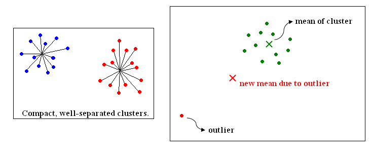
$ J=\sum _{j=1} ^{c} \sum _{X_i \in S_j}||X_i - \mu _ j||^2 $ (2-8)
where $ \mu _j = \frac{1}{|S_j|} \sum _{X_i \in S_j} X_i $ (2-9)
- Good when clusters are compact, well separated
- Sensitive to outliers
$ J=\sum _{j=1} ^{c} \sum _{X_i \in S_j} ||X_i - \mu_j||_{L1} $ is more robust to outliers
Can use other types of similarity measure
$ S(X_1, X_2)=\frac{X_1 \cdot X_2}{||X_1||||X_2||} $ (2-10)
to speed up optimization of J
Use "Nearest mean reclassification rule"
- choose initial partition $ S_1, S_2 , \cdots , S_c $ (2-11)
- calculate $ \mu _1 , \mu _2 , \cdots , \mu _c $
- reclsssify each $ X_i $ to the class of the nearest mean
- If cluster have changed, repeat
Note: $ X_i $ class of its nearest mean
is same as choosing the move for $ X_i $ that moves $ \Delta J $ as negative as possible because $ J=\sum _{j=1} ^{c} \sum _{X_i \in S_j} ||X_i - \mu _j||^2 $ (2-12)
If $ X_{io} \in S_{jo} \rightarrow X_{io} \in S_{\bar{j0}} $,
$ J \Rightarrow \sum _{j=1} ^{c} \sum _{X_i \in S_j} ||X_i - \mu_j||^2 - ||X_{io}-\mu _{jo}||^2 + ||X_{io} - \mu _{\bar {jo}}||^2 $ (2-13)
$ \Delta J $ is as negative as possible when $ ||X_{io} - \mu _{\bar {jo}}||^2 $ is $ \begin{smallmatrix} min\\ j \end{smallmatrix} ||X_i -\mu _j||^2 $ (2-14)
Can use FORGY, CLUSTER
Observation
$ J= \cdots = \sum _{j=1} ^c \frac{1}{|S_j|} \sum _{X_i \in S_j , X_k \in S_j} \frac{||X_i-X_k||^2}{2} $ (2-15)
This is a distance based clustering method.
No need for feature vector
Previous: Lecture 24 Next: Lecture 26


