| (16 intermediate revisions by 7 users not shown) | |||
| Line 1: | Line 1: | ||
| + | <center><font size= 4> | ||
| + | '''[[ECE662]]: Statistical Pattern Recognition and Decision Making Processes''' | ||
| + | </font size> | ||
| + | |||
| + | Spring 2008, [[user:mboutin|Prof. Boutin]] | ||
| + | |||
| + | [[Slectures|Slecture]] | ||
| + | |||
| + | <font size= 3> Collectively created by the students in [[ECE662:BoutinSpring08_OldKiwi|the class]]</font size> | ||
| + | </center> | ||
| + | |||
| + | ---- | ||
| + | =Lecture 22 Lecture notes= | ||
| + | Jump to: [[ECE662_Pattern_Recognition_Decision_Making_Processes_Spring2008_sLecture_collective|Outline]]| | ||
| + | [[Lecture 1 - Introduction_OldKiwi|1]]| | ||
| + | [[Lecture 2 - Decision Hypersurfaces_OldKiwi|2]]| | ||
| + | [[Lecture 3 - Bayes classification_OldKiwi|3]]| | ||
| + | [[Lecture 4 - Bayes Classification_OldKiwi|4]]| | ||
| + | [[Lecture 5 - Discriminant Functions_OldKiwi|5]]| | ||
| + | [[Lecture 6 - Discriminant Functions_OldKiwi|6]]| | ||
| + | [[Lecture 7 - MLE and BPE_OldKiwi|7]]| | ||
| + | [[Lecture 8 - MLE, BPE and Linear Discriminant Functions_OldKiwi|8]]| | ||
| + | [[Lecture 9 - Linear Discriminant Functions_OldKiwi|9]]| | ||
| + | [[Lecture 10 - Batch Perceptron and Fisher Linear Discriminant_OldKiwi|10]]| | ||
| + | [[Lecture 11 - Fischer's Linear Discriminant again_OldKiwi|11]]| | ||
| + | [[Lecture 12 - Support Vector Machine and Quadratic Optimization Problem_OldKiwi|12]]| | ||
| + | [[Lecture 13 - Kernel function for SVMs and ANNs introduction_OldKiwi|13]]| | ||
| + | [[Lecture 14 - ANNs, Non-parametric Density Estimation (Parzen Window)_OldKiwi|14]]| | ||
| + | [[Lecture 15 - Parzen Window Method_OldKiwi|15]]| | ||
| + | [[Lecture 16 - Parzen Window Method and K-nearest Neighbor Density Estimate_OldKiwi|16]]| | ||
| + | [[Lecture 17 - Nearest Neighbors Clarification Rule and Metrics_OldKiwi|17]]| | ||
| + | [[Lecture 18 - Nearest Neighbors Clarification Rule and Metrics(Continued)_OldKiwi|18]]| | ||
| + | [[Lecture 19 - Nearest Neighbor Error Rates_OldKiwi|19]]| | ||
| + | [[Lecture 20 - Density Estimation using Series Expansion and Decision Trees_OldKiwi|20]]| | ||
| + | [[Lecture 21 - Decision Trees(Continued)_OldKiwi|21]]| | ||
| + | [[Lecture 22 - Decision Trees and Clustering_OldKiwi|22]]| | ||
| + | [[Lecture 23 - Spanning Trees_OldKiwi|23]]| | ||
| + | [[Lecture 24 - Clustering and Hierarchical Clustering_OldKiwi|24]]| | ||
| + | [[Lecture 25 - Clustering Algorithms_OldKiwi|25]]| | ||
| + | [[Lecture 26 - Statistical Clustering Methods_OldKiwi|26]]| | ||
| + | [[Lecture 27 - Clustering by finding valleys of densities_OldKiwi|27]]| | ||
| + | [[Lecture 28 - Final lecture_OldKiwi|28]] | ||
| + | ---- | ||
| + | ---- | ||
Note: Most tree growing methods favor greatest impurity reduction near the root node. | Note: Most tree growing methods favor greatest impurity reduction near the root node. | ||
| − | + | Example: | |
[[Image:Lecture22_DecisionTree_OldKiwi.JPG]] Figure 1 | [[Image:Lecture22_DecisionTree_OldKiwi.JPG]] Figure 1 | ||
| Line 7: | Line 51: | ||
To assign category to a leaf node. | To assign category to a leaf node. | ||
| + | <source lang="matlab"> | ||
Easy! | Easy! | ||
| Line 16: | Line 61: | ||
-> assign the most frequent class. | -> assign the most frequent class. | ||
| + | </source> | ||
Note: Problem of building decision tree is "ill-conditioned" | Note: Problem of building decision tree is "ill-conditioned" | ||
| Line 21: | Line 67: | ||
i.e. small variance in the training data can yield large variations in decision rules obtained. | i.e. small variance in the training data can yield large variations in decision rules obtained. | ||
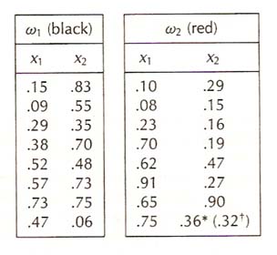
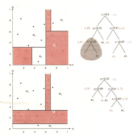
| − | Ex. p.405( | + | Ex. p.405(Duda & Hart) |
| + | |||
| + | [[Image:fig101_OldKiwi.jpg]] [[Image:fig102_OldKiwi.jpg]] | ||
A small move of one sample data can change the decision rules a lot. | A small move of one sample data can change the decision rules a lot. | ||
| − | + | == Clustering References == | |
"Data clustering, a review," A.K. Jain, M.N. Murty, P.J. Flynn[http://www.cs.rutgers.edu/~mlittman/courses/lightai03/jain99data.pdf] | "Data clustering, a review," A.K. Jain, M.N. Murty, P.J. Flynn[http://www.cs.rutgers.edu/~mlittman/courses/lightai03/jain99data.pdf] | ||
| Line 59: | Line 107: | ||
* Mixture of Gaussians(Probabilistic) | * Mixture of Gaussians(Probabilistic) | ||
| + | Here are some useful links for getting information & source about each clustering techniques. | ||
| + | |||
| + | * http://home.dei.polimi.it/matteucc/Clustering/tutorial_html/index.html | ||
| + | * http://mvhs.shodor.org/mvhsproj/clustering/MatClust2.html | ||
| + | * http://www.lottolab.org/DavidCorney/ClusteringMatlab.html | ||
| Line 95: | Line 148: | ||
Here is another example for image segmentation and compression from [http://research.microsoft.com/~cmbishop/prml/] | Here is another example for image segmentation and compression from [http://research.microsoft.com/~cmbishop/prml/] | ||
| − | |||
[[Image:k_means_OldKiwi.jpg]] | [[Image:k_means_OldKiwi.jpg]] | ||
| + | |||
| + | As can be seen, there is a trade-off between compression and image quality when the clustering is considered. The clustering is based on the similarity of colors. The most common color values are chosen to be k-means. Larger values of k increases the image quality while compression rate decrease. | ||
Input to a clustering algorithm is either | Input to a clustering algorithm is either | ||
| − | + | * distances between each pairs of objects in dataset | |
| + | |||
| + | * feature vectors for each object in dataset | ||
| + | ---- | ||
| + | Previous: [[Lecture_21_-_Decision_Trees(Continued)_OldKiwi|Lecture 21]] | ||
| + | Next: [[Lecture_23_-_Spanning_Trees_OldKiwi|Lecture 23]] | ||
| + | |||
| − | + | [[ECE662:BoutinSpring08_OldKiwi|Back to ECE662 Spring 2008 Prof. Boutin]] | |
| + | [[Category:ECE662]] | ||
| + | [[Category:decision theory]] | ||
| + | [[Category:lecture notes]] | ||
| + | [[Category:pattern recognition]] | ||
| + | [[Category:slecture]] | ||
Latest revision as of 11:23, 10 June 2013
ECE662: Statistical Pattern Recognition and Decision Making Processes
Spring 2008, Prof. Boutin
Collectively created by the students in the class
Contents
Lecture 22 Lecture notes
Jump to: Outline| 1| 2| 3| 4| 5| 6| 7| 8| 9| 10| 11| 12| 13| 14| 15| 16| 17| 18| 19| 20| 21| 22| 23| 24| 25| 26| 27| 28
Note: Most tree growing methods favor greatest impurity reduction near the root node.
Example:
To assign category to a leaf node.
Easy!

If sample data is pure

-> assign this class to leaf.

else

-> assign the most frequent class.
Note: Problem of building decision tree is "ill-conditioned"
i.e. small variance in the training data can yield large variations in decision rules obtained.
Ex. p.405(Duda & Hart)
A small move of one sample data can change the decision rules a lot.
Clustering References
"Data clustering, a review," A.K. Jain, M.N. Murty, P.J. Flynn[1]
"Algorithms for clustering data," A.K. Jain, R.C. Dibes[2]
"Support vector clustering," Ben-Hur, Horn, Siegelmann, Vapnik [3]
"Dynamic cluster formation using level set methods," Yip, Ding, Chan[4]
What is clustering?
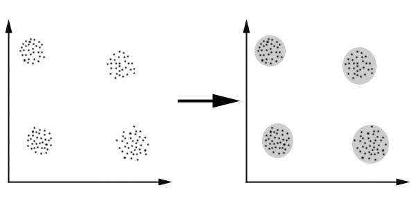
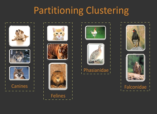
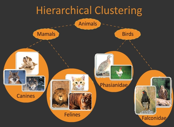
The task of finding "natural " groupings in a data set. Clustering is one of the most important unsupervised learning technique. Basically, it tries to find the structure of unlabeled data, that is, based on some distance measure, it tries to group the similar members. Here is a simple figure from [5]:
Clustering algorithms can also be classified as follows:
- Exclusive Clustering
- Overlapping Clustering
- Hierarchical Clustering
- Probabilistic Clustering
There are several clustering techniques, the most important ones are:\
- K-means Clustering(exclusive)
- Fuzzy C-means(Overlapping)
- Hierarchical clustering
- Mixture of Gaussians(Probabilistic)
Here are some useful links for getting information & source about each clustering techniques.
- http://home.dei.polimi.it/matteucc/Clustering/tutorial_html/index.html
- http://mvhs.shodor.org/mvhsproj/clustering/MatClust2.html
- http://www.lottolab.org/DavidCorney/ClusteringMatlab.html
Synonymons="unsupervised learning"
Clustering as a useful technique for searching in databases
Clustering can be used to construct an index for a large dataset to be searched quickly.
- Definition: An index is a data structure that enables sub-linear time look up.
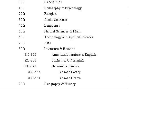
- Example: Dewey system to index books in a library
- Example of Index: Face Recognition
- need face images with label
- must cluster to obtain sub-linear search time
- Search will be faster because of $ \bigtriangleup $ inequality.
- Example: Image segmentation is a clustering problem
- dataset = pixels in image
- each cluster is an object in image
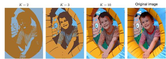
Here is another example for image segmentation and compression from [6]
As can be seen, there is a trade-off between compression and image quality when the clustering is considered. The clustering is based on the similarity of colors. The most common color values are chosen to be k-means. Larger values of k increases the image quality while compression rate decrease.
Input to a clustering algorithm is either
- distances between each pairs of objects in dataset
- feature vectors for each object in dataset
Previous: Lecture 21 Next: Lecture 23


