Create the page "Plot" on this wiki! See also the search results found.
- I will take the values from 0 to 2 seconds, repeat it every 2 seconds and plot it over three periods using the following MATLAB code: plot(t1,y1,t2,y2,t3,y3)1 KB (217 words) - 08:58, 12 September 2008
- plot(t,x)296 B (51 words) - 09:32, 12 September 2008
- %The following code attempts to plot 13 cycles of plot(t,x,'--r')718 B (119 words) - 10:41, 12 September 2008
- plot(t,x).434 B (59 words) - 10:46, 12 September 2008
- ...rtmann. I use period of 10 to create this signal to be a periodic one. The plot is shown below:310 B (57 words) - 11:05, 12 September 2008
- plot(t,x) plot(t,x)1,020 B (176 words) - 11:10, 12 September 2008
- plot(t,x)402 B (73 words) - 11:14, 12 September 2008
- plot(t,x) plot(t,x)775 B (125 words) - 17:10, 12 September 2008
- plot(x,y)"851 B (147 words) - 15:14, 12 September 2008
- An easy way to prove if a system is linear is to plot the equation representing the system and then draw a horizontal line, i.e.1 KB (197 words) - 13:16, 12 September 2008
- plot(t,x);411 B (70 words) - 12:57, 12 September 2008
- plot(t,x) plot(t,x)260 B (50 words) - 15:25, 12 September 2008
- plot(t, x);389 B (59 words) - 13:38, 12 September 2008
- ...uses Ts of 0.07, or a '''sampling rate''' of 0.07 seconds. Therefore, the plot appears to only show one cycle of the sinusoid. plot(t,x);</pre>545 B (94 words) - 14:05, 12 September 2008
- ...ere is uite large, as a result it is not getting enough points in order to plot a proper garph. plot(t,x)398 B (72 words) - 14:44, 12 September 2008
- plot(n,y) plot(n,y2)769 B (126 words) - 15:32, 12 September 2008
- plot(x,y)499 B (90 words) - 15:14, 12 September 2008
- plot(t,x) plot(t,x)380 B (70 words) - 15:31, 12 September 2008
- plot(t,x)371 B (59 words) - 15:35, 12 September 2008
- original plot: plot(t,y,'b-')649 B (104 words) - 16:13, 12 September 2008
- plot(t,x) plot(t,x)431 B (76 words) - 15:55, 12 September 2008
- plot(t,x) plot(t,y)939 B (153 words) - 18:26, 12 September 2008
- plot(t,x) plot(t,x)594 B (85 words) - 17:38, 12 September 2008
- plot(t,x);445 B (77 words) - 18:20, 12 September 2008
- The following plot shows two periods of the periodic DT signal <math>x[n]</math>, a sawtooth: From the plot above, N = 4:1 KB (162 words) - 13:40, 24 September 2008
- We will first find the fourrier transform X(W) and plot out its signal over a period of frequency Wm.805 B (160 words) - 20:06, 17 November 2008
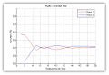
File:Hca Old Kiwi.jpg Plot about the accuracy of Bayes Classification system for the data in Hcd.jpg.(642 × 442 (40 KB)) - 05:25, 26 May 2009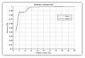
File:Mca Old Kiwi.jpg Plot about the accuracy of Bayes Classification system for the data in Lcd.jpg.(641 × 441 (38 KB)) - 05:25, 26 May 2009- All points which satisfy D(X,0)=k, for some Constant k, if we plot them we will get a sphere.3 KB (528 words) - 08:48, 10 April 2008
- Then, for each threshold, you plot the [[true positive rate_Old Kiwi]] against the [[false positive rate_Old K3 KB (621 words) - 08:48, 10 April 2008
- ...nima status with some other points, and this is shown below in the contour plot by the small line.2 KB (336 words) - 14:53, 16 March 2008
- plot(r(:,1),r(:,2),'.');2 KB (362 words) - 17:44, 19 March 2008
- ...ctly with this command. However, this information is needed to derive (and plot) the theoretical expression for tex:S_y(e^{-j\mu}, e^{-j\nu}). Use the fact2 KB (258 words) - 00:51, 22 March 2008
- subplot(length(n), length(h1), (row-1)*length(h1)+col); plot(x,prob_estimate);2 KB (267 words) - 20:45, 26 March 2008
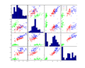
File:Iris Old Kiwi.png Scatter-plot of Fisher's Iris Flower Dataset.(1,060 × 846 (24 KB)) - 05:25, 26 May 2009- First plot shows the actual classes of the dataset, second plot shows the situation in which we do not know the label of the data points, a888 B (147 words) - 15:11, 24 April 2008
- [Plot of solution]710 B (117 words) - 12:19, 22 October 2010
- Express each of the following complex numbers in polar form, and plot them in the complex plane, indicating the magnitude and angle of each numbe1 KB (232 words) - 01:33, 13 June 2008
- ...e two. I think this is how you do it at least. I am going to use MATLAB to plot them. --[[User:Kfernan|Kevin Fernandes]]3 KB (560 words) - 05:47, 30 September 2009
- *Be sure to get the full story on the dirac function, convolution, bode plot approximations, and linearity. Don't rely on memorization. -Mike7 KB (1,297 words) - 11:41, 10 December 2011
- plot(t,sin(t)); plot(t,noise);7 KB (1,251 words) - 11:54, 21 September 2012
- ...z1 by r1.exp(jw1), where r1 and w1 are constants. Now, for an approximate plot, do I fix r1 and w1, as the values that correspond to the approximate locat4 KB (628 words) - 15:47, 30 November 2010
- ...tion. We will look at the signal in the frequency domain, as shown in the plot below: As seen in the plot, the signal <math> X(f) </math> has a triangular shape and is band-limited5 KB (840 words) - 19:08, 22 September 2009
- Let us assume the following plot for <math>X_1(\omega)</math>. We will also assume that the Nyquist conditio Now, on scaling we have the following plot for <math>\frac{1}{D} X_1(\frac{\omega}{D})</math>4 KB (655 words) - 07:13, 23 September 2009
- ...olors (along a set color scale) or varying shades of black for a grayscale plot. An example of each type is shown below:8 KB (1,268 words) - 07:16, 23 September 2009
- ...ously, the signal now contains more samples, as we can see from the x-axis plot.5 KB (847 words) - 11:54, 21 September 2012
- han = plot(time,x); han1 = plot(f,abs(X));780 B (113 words) - 20:52, 13 October 2009
- han = plot(time,x); han1 = plot(f,abs(X));3 KB (343 words) - 21:04, 14 October 2009
- han = plot(time,bear); han1 = plot(f,abs(BEAR));2 KB (232 words) - 21:55, 14 October 2009
- ...sity.Generally Spectrograms are done in gray scale,where the darkness of a plot represents the high intensity regions.2 KB (356 words) - 06:07, 23 September 2014