Back to all ECE 600 notes
Previous Topic: Random Variables: Definitions
Next Topic: Conditional Distributions
The Comer Lectures on Random Variables and Signals
Topic 6: Random Variables: Distributions
How do we find, compute and model P(x ∈ A) for a random variable X for all A ∈ B(R)? We use three different functions:
- the cumulative distribution function (cdf)
- the probability density function (pdf)
- the probability mass function (pmf)
We will discuss these in this order, although we could come at this discussion in a different way and a different order and arrive at the same place.
Definition $ \quad $ The cumulative distribution function (cdf) of X is defined as
Notation $ \quad $ Normally, we write this as
So $ F_X(x) $ tells us P$ P_X(A) $ if A = (-∞,x] for some real x.
What about other A ∈ B(R)? It can be shown that any A ∈ B(R) can be written as a countable sequence of set operations (unions, intersections, complements) on intervals of the form (-∞,x$ _n $], so can use the probability axioms to find $ P_X(A) $ from $ F_X $ for any A ∈ B(R). This is not how we do things in practice normally. This will be discussed more later.
Can an arbitrary function $ F_X, $ be a valid cdf? No, it cannot.
Properties of a valid cdf:
1.
This is because
and
2. For any $ x_1,x_2 $ ∈ R such that $ x_1<x_2 $,
i.e. $ F_X(x) $ is a non decreasing function.
3. $ F_X $ is continuous from the right , i.e.
Proof:
First, we need some results from analysis and measure theory:
(i) For a sequence of sets, $ A_1, A_2,... $, if $ A_1 $ ⊃ $ A_2 $ ⊃ ..., then
(ii) If $ A_1 $ ⊃ $ A_2 $ ⊃ ..., then
(iii) We can write $ F_X(x^+) $ as
Now let
Then
4. $ P(X>x) = 1-F_X(x) $ for all x ∈ R
5. If $ x_1 < x_2 $, then
6. $ P(\{X=x\})= F_X(x) - F_X(x^-) $, where
Contents
- 1 The Probability Density Function
- 2 Continuous and Discrete Random Variables
- 3 Probability Mass Function
- 4 Some Important Random Variables
- 5 1. Gaussian Random Variable
- 6 2. Uniform Random Variable
- 7 3. Binomial Random Variable (Disrete)
- 8 4. Exponential (Continuous)
- 9 5. Rayleigh (Continuous)
- 10 6. Laplace (Continuous)
- 11 7. Poisson (Discrete)
- 12 8. Geometric (Discrete)
- 13 References
- 14 Questions and comments
The Probability Density Function
Definition $ \quad $ The probability density function (pdf) of a random variable X is the derivative of the cdf of X,
at points where $ F_x $ is differentiable.
From the Fundamental Theorem of Calculus, we then have that
Important note: the cdf $ F_X $ might not be differentiable everywhere. At points where $ F_X $ is not differentiable, we can use the Dirac delta function to defing $ f_x $.
Definition $ \quad $ The Dirac Delta Function $ \delta(x) $ is the function satisfying the properties:
1.
2.
If $ F_X $ is not differentiable at a point, use $ \delta(x) $ at that point to represent $ f_X $.
Why do we do this? Consider the step function $ u(x) $, which is discontinuous and thus not differentiable at $ x=0 $. This is a common type of discontinuity we see in cdfs. The derivative of $ u(x) $ is defined as
This limit does not exist at $ x=0 $
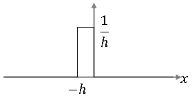
Let's look at the function
It looks like this:
For any x ≠ 0, we have that
for small enough h.
Also, ∀ $ \epsilon $ > 0,
So, in the limit, the function g(x) has the properties of the $ \delta $-function as h tends to 0. A similar argument can be made for h<0.
So this is why it is sometimes written that
Since we will only work with non-differentiable functions that have step discontinuities as cdfs, we write
with the understanding that $ d/dx $ is not necessarily the traditional definition of the derivative.
Properties of the pdf:
1. (proof: derivative of increasing Function F$ _X $(x) must be non-negative)
2. (proof: use the fact that the limit of F$ _X $(x) as x goes to infinity is 1)
3. If $ x_1<x_2 $, then
- (proof: use the fact that P(x$ _1 $ < X ≤ x$ _2 $) = F$ _X $(x$ _2 $) - F$ _X $(x$ _1 $))
Some notes:
- We introduced the concept of a pdf in our discussion of probability spaces. We could have defined the pdf of a random variable X as a function $ f_X $ satisfying properties 1 and 2 above, and then define $ F_X $ in terms of $ f_X $.
- f_X(x) is not a probability for a fixed x, it gives us instead the "probability density", so it must be integrated to give us the probability.
- In practice, to compute probabilities of random variable X, we normally use
Continuous and Discrete Random Variables
A random variable X having a cdf that is continuous everywhere is called a continuous random variable.
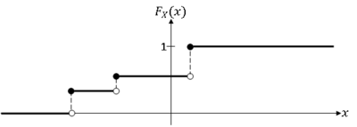
A random variable X having a piece-wise constant cdf is a discrete random variable.
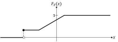
A random variable X whose cdf is neither continuous everywhere nor piece-wise constant is a mixed random variable.
We will consider only discrete and continuous random variables in this course.
Note:
- For a continuous random variable X, P(X=x)=0 ∀x ∈ R, because $ F_X(x)-F_X(x^-) = 0 $ ∀x ∈ R.
- We can use the cdf/pdf functions for a discrete random variable X, but generally, we do not. Instead, we use the pmf.
Probability Mass Function
The probability mass function (pmf) of random variable X is the function
We will use this function when X is discrete.
Although P(X=x) exists for every x ∈ R, we normally define $ p_X(x) $ for some subset R⊂R
Definition $ \quad $ Given random variable X:S→R, let R = X(S) be the range space of X (note that the range of X is still R).
Example: Let X be the sum of values rolled on two fair die. Then R = {2,3,...,12}.
We define the pmf only on R, so in the example above, we would have $ p_X(x) = P(X=x) $ ∀x ∈ R.
We can now consider the probability space for a discrete random variable to be (R,P(R),p$ _X $).
Note that if X is continuous, we define the cdf/pdf for all x ∈ R. for example, if X = V$ ^2 $, where V is the voltage (so X is proportional to power), then R=[0,∞), but we still define $ f_X(x) $ ∀x ∈ R.
Properties of the pmf:
1. (proof)
2. (proof)
These properties can be derived from the axioms. Note that we could simply define the pmf to be a function having these two and then create a probability mapping P(.) in such a way that P(.) will satisfy the axioms. We discussed this in our lectures on probability spaces. This is what we do in practice.
Some Important Random Variables
1. Gaussian Random Variable
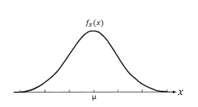
The Gaussian (or Normal) continuous random variable $ X $ has pdf
and cdf $ F_X(x) $, where
(No closed solution)
Let
Then write
Use the table to find values of ϕ.
Notation for Gaussian random variable $ X $:$ N(\mu,\sigma^2) $
Gaussian random variable are used to model
- certain types of noise
- sum of large number of independent random variables
- continuous random variables with no prior information about distribution (default assumption)
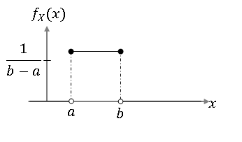
2. Uniform Random Variable
Continuous Case:
Discrete Case
$ R = \{x_1,...,x_2\} $ for some integer n ≥ 1.
Used to model:
- Continuous case - random variables where $ P(X $∈(a,b)) depends only on $ b-a $, ∀a,b ∈ R, $ x_1 $≤a<b≤$ x_2 $
- Discrete case - random variables whose values are equally likely to occur.
3. Binomial Random Variable (Disrete)
$ R = \{0,1,...,n\} $
p ∈ [0,1], n ≥ 1, n finite.
Used to model number of successes in Bernoulli trials
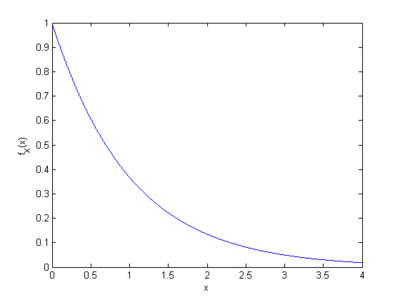
4. Exponential (Continuous)
Used to model
- times between arrival of customers (or other things)
- lifetimes of devices/systems
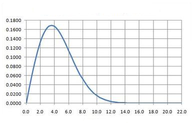
5. Rayleigh (Continuous)
Used to model square root of a sum of squares (e.g. magnitude of complex exponential).
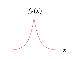
6. Laplace (Continuous)
Used to model prediction errors.
7. Poisson (Discrete)
Used to model the number of occurrences of events in time or space.
8. Geometric (Discrete)
Form 1:
Form 2:
Used to model number of Bernoulli trials until the occurrence of first success.
References
- M. Comer. ECE 600. Class Lecture. Random Variables and Signals. Faculty of Electrical Engineering, Purdue University. Fall 2013.
Questions and comments
If you have any questions, comments, etc. please post them on this page
Back to all ECE 600 notes
Previous Topic: Random Variables: Definitions
Next Topic: Conditional Distributions

