ECE600 F13 rv conditional distribution mhossain - Rhea

Topic 7: Random Variables: Conditional Distributions

We will now learn how to represent conditional probabilities using the cdf/pdf/pmf. This will provide us some of the most powerful tools for working with random variables: the conditional pdf and conditional pmf.

Recall that

P(A|B) = \frac{P(A\cap B)}{P(B)}

∀ A,B ∈ F with P(B) > 0.

We will consider this conditional probability when A = {X≤x} for a continuous random variable or A = {X=x} for a discrete random variable.

Discrete X

If P(B)>0, then let

P_X(x|B)\equiv P(X=x|B)=\frac{p(\{X=x\}\cap B)}{P(B)}

∀x ∈ R, for a given B ∈ F.
The function p $$ _X $$ is the conditional pmf of X. Recall Bayes' theorem and the Total Probability Law:

P(A|B)=\frac{P(B|A)P(A)}{P(B)};\quad P(B), P(A)>0

and

P(B)=\sum_{i = 1}^nP(B|A_i)P(A_i)

if $$ A_1,...,A_n $$ form a partition of S and $$ P(A_i)>0 $$ ∀i.

In the case A = {X=x}, we get

p_X(x|B) = \frac{P(B|X=x)p_X(x)}{P(B)}

where p $$ _X $$ (x|B) is the conditional pmf of X given B and $$ p_X(x) $$ is the pmf of X. Note that Bayes' Theorem in this context requires not only that P(B) >0 but also that P(X = x) > 0.

We also can use the TPL to get

p_X(x) = \sum_{i=1}^n p_X(x|A_i)P(A_i)

Continuous X

Let A = {X≤x}. Then if P(B)>0, B ∈ F, define

F_X(x|B)\equiv P(X\leq x|B) = \frac{P(\{X\leq x\}\cap B)}{P(B)}

as the conditional cdf of X given B.
The conditional pdf of X given B is then

f_X(x|B) = \frac{d}{dx}F_X(x|B)

Note that B may be an event involving X.

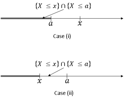
Example: let B = {X ≤ a} for some a ∈ R. Then

F_X(x|B) = \frac{P(\{X\leq x\}\cap\{X\leq a\})}{P(X\leq a)}

Two cases:

Case (i): $$ x > a $$

F_X(x|B) = \frac{P(X\leq a)}{P(X\leq a)} = 1

Case (ii): $$ x < a $$

F_X(x|B) = \frac{P(X\leq x)}{P(X\leq a)} = \frac{F_X(x)}{F_X(a)}

Fig 1: {X ≤ x} ∩ {X ≤ a} for the two different cases.

Now,

f_X(x|B) = f_X(x|X\leq a)=\begin{cases} 0 & x>a \\ \frac{f_X(x)}{F_X(a)} & x\leq a \end{cases}

Fig 2: f

$ _X $

(x) and f

$ _X $

(x

$ | $

X ≤ a).

Bayes' Theorem for continuous X:
We can easily see that

F_X(x|B)= \frac{P(B|X\leq x)F_X(x)}{P(B)}

from previous version of Bayes' Theorem, and that

F_X(x)=\sum_{i=1}^n F_X(x|A_i)P(A_i)

if $$ A_1,...,A_n $$ form a partition of S and P( $$ A_i $$ ) > 0 ∀ $$ i $$ , from TPL.
but what we often want to know is a probability of the type P(A|X=x) for some A∈F. We could define this as

P(A|X=x)\equiv\frac{P(A\cap \{X=x\})}{P(X=x)}

but the right hand side (rhs) would be 0/0 since X is continuous.
Instead, we will use the following definition in this case:

P(A|X=a)\equiv\lim_{\Delta x\rightarrow 0}P(A|x<X\leq x+\Delta x)

\Delta x > 0 \

using our standard definition of conditional probability for the rhs. This leads to the following derivation:

\begin{align} P(A|X=x) &= \lim_{\Delta x\rightarrow 0}\frac{P(x<X\leq x+\Delta x|A)P(A)}{P(x<X\leq x+\Delta x)} \\ \\ &= P(A)\lim_{\Delta x\rightarrow 0}\frac{F_X(x+\Delta x|A)-F_X(x|A)}{F_X(x+\Delta x)-F_X(x)} \\ \\ &= P(A)\frac{\lim_{\Delta x\rightarrow 0}\frac{F_X(x+\Delta x|A)-F_X(x|A)}{\Delta x}}{\lim_{\Delta x\rightarrow 0}\frac{F_X(x+\Delta x)-F_X(x)}{\Delta x}}\\ \\ &=P(A)\frac{f_X(x|A)}{f_X(x)} \end{align}

So,

P(A|X=x)=\frac{f_X(x|A)P(A)}{f_X(x)}

This is how Bayes' Theorem is normally stated for a continuous random variable X and an event A∈F with P(A) > 0.

We will revisit Bayes' Theorem one more time when we discuss conditional distributions for two random variables.

References

M. Comer. ECE 600. Class Lecture. Random Variables and Signals. Faculty of Electrical Engineering, Purdue University. Fall 2013.

Questions and comments

If you have any questions, comments, etc. please post them on this page

Back to all ECE 600 notes
Previous Topic: Random Variables: Distributions
Next Topic: Functions of a Random Variable

ECE600 F13 rv conditional distribution mhossain - Rhea

Contents

Discrete X

Continuous X

References

Questions and comments

Alumni Liaison