ECE600 F13 rv Functions of random variable mhossain - Rhea

Topic 8: Functions of Random Variables

We often do not work with the random variable we observe directly, but with some function of that random variable. So, instead of working with a random variable X, we might instead have some random variable Y=g(X) for some function g:R → R.
In this case, we might model Y directly to get f $$ _Y $$ (y), especially if we do not know g. Or we might have a model for X and find f $$ _Y $$ (y) (or p $$ _Y $$ (y)) as a function of f $$ _X $$ (or p $$ _X $$ and g.
We will discuss the latter approach here.

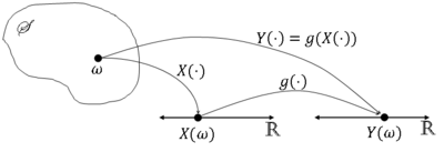
More formally, let X be a random variable on (S,F,P) and consider a mapping g:R → R. Then let Y $(\omega)=$ g(X( $\omega))$ ∀ $\omega$ ∈ S.
We normally write this as Y=g(X).

Graphically,

Fig 1: Mapping from S to X to Y under g

Is Y a random variable? We must have Y $^{-1}$ (A) ≡ { $\omega$ ∈ S: Y $(\omega)$ ∈ A} = { $\omega$ ∈ S: g(X $(\omega)$ ) ∈ A} be an element of F ∀A ∈ B(R) (Y must be Borel measurable).
We will only consider functions g in this class for which Y $^{-1}$ (A) ∈ F ∀A ∈ B(R), so that if Y=g(X) for some random variable X, Y will be a random variable.

What is the distribution of Y? Consider 3 cases:

X discrete, Y discrete
X continuous, Y discrete
X continuous, Y continuous

Note: you cannot have a continuous Y from a discrete X.

Case 1: X and Y Discrete

Let $$ R_X $$ ≡ X(S) be the range space of X and $$ R_Y $$ ≡ g(X(S)) be the range space of Y (i.e. the image of X(S) under g). Then the pmf of Y is

p

$ _Y $

(y) = P(Y=y) = P(g(X)=y)

But this means that

p_Y(y) = \sum_{x\in\mathcal{R}_X:g(x)=y}p_X(x)\;\;\forall y\in\mathcal{R}_Y

Example $\quad$ Let X be the value rolled on a die and

Y = \begin{cases} 1 & \mbox{if}\;X\;\mbox{is odd} \\ 0 & \mbox{if}\;X\;\mbox{is even} \end{cases}

Then R $$ _X $$ = {0,1,2,3,4,5,6} and R $$ _Y $$ = {0,1} and g(x) = x % 2.

Now

p_Y(y) = \sum_{x\in\mathcal{R}_X:g(x)=y}p_X(x)

\begin{align} \Rightarrow p_Y(0) &= p_X(2)+p_X(4)+p_X(6) \\ p_Y(1) &= p_X(1)+p_X(3)+p_X(5) \end{align}

Case 2: X Continuous, Y Discrete

The pmf of Y in this case is

p

$ _Y $

(y) = P(g(X)=y) = P(X ∈ D

$ _y $

)
where D

$ _y $

≡ {x ∈ R: g(x)=y} ∀y ∈ R

$ _y $

i.e. for a given y ∈ R $$ _y $$ , D $$ _y $$ is the set of all x ∈ R such that g(x) = y.

Then,

p_Y(y) = \int_{D_y}f_X(x)dx

Example Let g(x) = u(x - x $$ _0 $$ ) for some x $$ _0 $$ ∈ R, and let Y=g(X). Then $$ R_Y $$ = {0,1} and

D

$ _0 $

= {x ∈ R: x < x

$ _0 $

} = (-∞, x

$ _0 $

) D

$ _1 $

= {x ∈ R: x ≥ x

$ _0 $

} = [ x

$ _0 $

, ∞)

So,

p_Y(y) = \begin{cases} \int_{-\infty}^{x_0} f_X(x)dx & y=0\\ \\ \int_{x_0}^{-\infty} f_X(x)dx & y=1 \end{cases}

Case 3: X and Y Continuous

We will discuss 2 methods for finding f $$ _Y $$ in this case.

Approach 1
First, find the cdf F $$ _Y $$ .

F

$ _Y $

(y) = P(g(X) ≤ y) = P(X ∈ D

$ _y $

)
where D

$ _y $

= {x ∈ R: g(x) ≤ y}.

i.e. for a given y ∈ R, D $$ _y $$ is the set of all x ∈ R such that g(x) ≤ y.

Then

F_Y(f) = \int_{D_y}f_X(x)dx

Differentiate F $$ _Y $$ to get f $$ _y $$ .

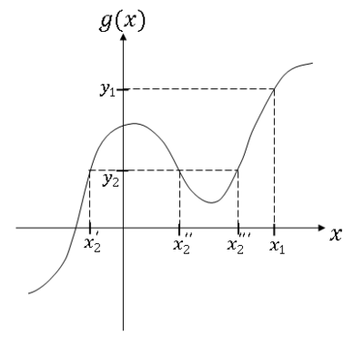
You can find D $$ _Y $$ graphically or analytically

Example

Fig 2: This plot of g(x) can be used to derive D

$ _Y $

graphically

For y = y $$ _1 $$ and y = y $$ _2 $$ ,

\begin{align} D_{y_1} &= \{x:\;x \leq x_1\} \\ D_{y_2} &= \{x:\;x\leq x_2'\} \cup \{x:\;x_2''<x\leq x_2'''\} \end{align}

Then

\begin{align} F_Y(y_1) &= \int_{-\infty}^{x_1}f_X(x)dx \\ \\ F_Y(y_2) &= \int_{-\infty}^{x_2'}f_X(x)dx + \int_{x_2''}^{x_2'''}f_X(x)dx \end{align}

Example Y = aX + b, a,b ∈ R, a ≠ 0

F

$ _Y $

(y) = P(aX + b ≤ y)

So,

\begin{align} D_y&=\{x\in\mathbb R: x\leq\frac{y-b}{a}\}\quad\mbox{if}\;a>0 \\ D_y&=\{x\in\mathbb R: x\geq\frac{y-b}{a}\}\quad\mbox{if}\;a<0 \end{align}

Then

F_Y(y)=\begin{cases} \int_{-\infty}^{\frac{y-b}{a}}f_X(x)dx & \mbox{if }\;a>0 \\ \\ \int_{\frac{y-b}{a}}^{-\infty}f_X(x)dx & \mbox{if }\;a<0 \end{cases}

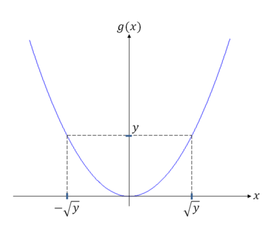
Example Y = X $$ ^2 $$

Fig 3: Y = X

$ ^2 $

For y < 0, D $$ _y $$ = ø
For y ≥ 0,

\begin{align} F_Y(y) &= P(X^2\leq y) \\ &= P(-\sqrt{y} <X\leq \sqrt{y}) \end{align}

So,

D_y = (-\sqrt{y},\sqrt{y})

and

F_Y(y) = \int_{-\sqrt{y}}^{\sqrt{y}}f_X(x)dx

For general y, we need to find subsets of the y-axis that have solutions of the same form and solve the problems separately for the different subsets.

Approach 2

Use a formula for f $$ _y $$ in terms of f $$ _X $$ . To derive the formula, assume the inverse function g $^{-1}$ exists, so if y = g(x), then x = g $^{-1}$ (y). Also assume g and g $^{-1}$ are differentiable. Then, if Y = g(X), we have that

f_Y(y) = \frac{f_X(g^{-1}(y))}{|\frac{dy}{dx}|_{x=g^{-1}(y)}}

Proof:
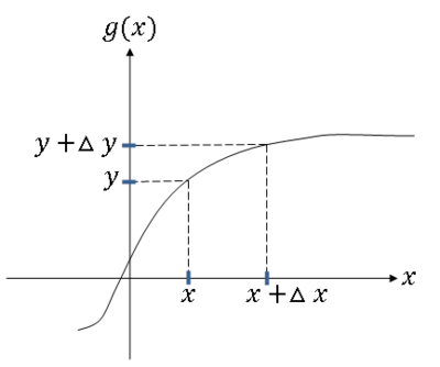
First consider g monotone (strictly monotone) increasing (note that for differentiable and hence continuous functions defined for a given interval, injection implies monotonicity, hence it is sufficient to limit our analysis to monotonic functions only).

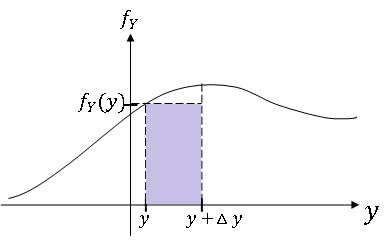
Fig 4: Function g is strictly increasing on its domain.

Since {y < Y ≤ y + Δy} = {x < X ≤ x + Δx}, we have that P(y < Y ≤ y + Δy) = P(x < X ≤ x + Δx).

Use the following approximations:

P(y < Y ≤ y + Δy) ≈ f $$ _Y $$ (y)Δy
P(x < X ≤ x + Δx) ≈ f $$ _X $$ (x)Δx

Fig 5: P(y < Y ≤ y + Δy) ≈ f

$ _Y $

(y)Δy

Since the left hand sides are equal,

f_Y(y)\Delta y \approx f_X(x)\Delta x

Now as Δy → 0, we also have that Δx → 0 since g is continuous, and the approximations above become equalities. We rename Δy, Δx as dy and dx respectively, so letting Δy → 0, we get

\begin{align} f_Y(y)dy &= f_X(x)dx \\ \Rightarrow f_Y(y)&=f_X(x)\frac{dx}{dy} \end{align}

We normally write this as

f_Y(y) = \frac{f_X(g^{-1}(y))}{\frac{dy}{dx}|_{x=g^{-1}(y)}}

A similar derivation for g monotone decreasing gives us the general result for invertible g:

f_Y(y) = \frac{f_X(g^{-1}(y))}{|\frac{dy}{dx}|_{x=g^{-1}(y)}}

Note this result can be extended to the case where y = g(x) has n solutions x $$ _1 $$ ,...,x $$ _n $$ , in which case,

f_Y(y) = \sum_{i=1}^n\frac{f_X(x_i)}{|\frac{dy}{dx}|_{x=x_i}}

For example, if Y = X $$ ^2 $$ ,

x_1 = -\sqrt{y},\;\;x_2 = \sqrt{y}

\Rightarrow f_Y(y) = \frac{f_X(-\sqrt{y})}{2\sqrt{y}}+\frac{f_X(\sqrt{y})}{2\sqrt{y}}

References

M. Comer. ECE 600. Class Lecture. Random Variables and Signals. Faculty of Electrical Engineering, Purdue University. Fall 2013.

Questions and comments

If you have any questions, comments, etc. please post them on this page

Back to all ECE 600 notes
Previous Topic: Conditional Distributions
Next Topic: Expectation

ECE600 F13 rv Functions of random variable mhossain - Rhea

Contents

Case 1: X and Y Discrete

Case 2: X Continuous, Y Discrete

Case 3: X and Y Continuous

References

Questions and comments

Alumni Liaison