ECE600 F13 rv definition mhossain - Rhea

Topic 5: Random Variables: Definition

Random Variables

So far, we have been dealing with sets. But as engineers, we work with numbers, variables, vectors, functions, signals, etc. We will spend the rest of the course learning about random variables, vectors, sequences, and processes, since these usually serve us better as engineers in practice. However, we will link each of these topics to a probability space, since probability spaces tie everything together.

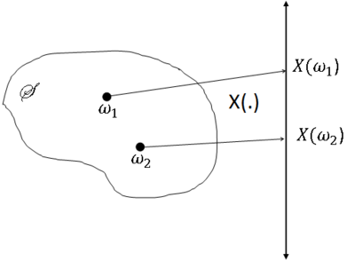
Informally, a random variable, often abbreviated to rv, is a function mapping the sample space S to the reals. However, we will restrict this function to lie within a certain class of functions.

First we present some definitions that will be needed.

Definition $\quad$ Given two spaces S and R, an R-valued function or mapping $$ f $$ :S→R assigns each element in S a value in R, so

f(\omega)\in\mathcal R \; \forall \omega \in \mathcal S

Definition $\quad$ Given any F ⊂ S and G ⊂ R, the image of F under $$ f $$ is

f(F)=\{a\in\mathcal R:\;a=f(\omega)\;\mbox{for some}\;\omega\in F\}

and the inverse image of G under $$ f $$ is

f^{-1}(G)=\{\omega\in\mathcal S:\;f(\omega) \in G\}

Note the following

$$ f $$ (F) is the set of all values in R that are mapped to by some element in F
$f^{-1}$ (G) is the set of all values in S that map to some value in G
The inverse image, $f^{-1}$ (G), is not the same as the inverse function $f^{-1}$ (a), a ∈ R.
$f(\omega)$ , $\omega$ ∈ S, is an element of R; $$ f $$ (F), F ⊂ S, is a subset of R.
$f^{-1}$ (a), a ∈ R, is an element of S; $f^{-1}$ (G), G ⊂ R, is a subset of S.
The inverse function $f^{-1}$ (a) ∀a ∈ R, may not exist. The inverse image $f^{-1}$ (G), G ⊂ R, always exists.

Definition of Random Variable (Beta version)
Given a probability space (S,F,P), a random variable is a function from S to the real line,

X:\mathcal S\rightarrow\mathbb R

Fig 1: Mapping elements of S to the real number line

In order to assign probabilities to events related to X, we will define a new probability space (R,B(R),P $$ _x $$ ), representing an "experiment" where the value of X is the outcome. Since $X(\omega)$ ∈ R ∀ $\omega$ ∈ S, our sample space is R. we always use the Borel field as the event space in this case.

What should P $$ _X $$ be? We need to define P $$ _X $$ (A) ∀ A ∈ R, where P $$ _X $$ (A)is the probability of event A in out new probability space. Since we can view the value of X as our outcome in this space, A occurs if X ∈ A, so P $$ _X $$ (A) is the probability that $X(\omega)$ ∈ A. Now,

\begin{align} \{X(\omega)\in A\} &= \{ \omega\in\mathcal S:\;X(\omega)\in A \} \\ &=X^{-1}(A) \\ \Rightarrow P_X(A) &= P(X^{-1}(A))\quad \forall A\in B(\mathbb R) \end{align}

but this requires that

X^{-1}(A) \in \mathcal F \quad \forall A\in B(\mathbb R)

This leads us to

Random Variable Definition 1
Given (S,F,P), a random variable is a mapping X:S→R with property that

X^{-1}(A) \equiv \{\omega\in\mathcal S :\; X(\omega)\in A\}\in \mathcal F\quad \forall A\in B(\mathbb R)

X:S→R satisfying this property is called a Borel measurable function. With this property, we can let

P_X(A) = P(X^{-1}(A))\quad \forall A\in B(\mathbb R)

It can be shown that X(.) is measurable if it is:

continuous
an indicator function $I_A(\omega)$ for some A ∈ B(R)
the limit of a sequence of measurable function: i.e. for $$ X_n $$ measurable for all n = 1,2,...

X(\omega) = \lim_{n\rightarrow\infty}X_n(\omega)

A countable sum of measurable functions

Note that if a function belongs to one or more of the four categories listed above then we can say that the function is measurable but it is not a necessary condition (if but not iff).

An example of a non measurable function: let S=R and F ⊂ S where F = P(R)-B(R), i.e. the set difference between the power set of R and its Borel field. So F ∉ B(R). Then, $X(\omega) = I_F(\omega)$ is not measurable. To see this, note that

X(\omega) = \begin{cases} 1 & \mbox{if }\omega\in F \\ 0 & \mbox{else} \end{cases}

and consider A={1} ∈ B(R).
Then

X^{-1}= F \notin \mathcal F = B(\mathbb R)

We will use definition 1 of a random variable in this class. Then we can let

P_X(A) = P(X^{-1}(A))\;\;\forall A\in B(\mathbb R)

Notation

P_X(A) = P(X\in A) = P(\{\omega \in \mathcal S:\; X(\omega)\in A\})

So A is an event in the Borel field in the probability soace (R,B(R),P $$ _X $$ ). But {X ∈ A} = { $\omega$ ∈ S: X( $\omega$ ) ∈ A} is an event in F.

In practice, how do we find P(X ∈ A)? the answer depends on whether X ia a discrete or continuous random variable, which we discuss next in Distributions.

References

M. Comer. ECE 600. Class Lecture. Random Variables and Signals. Faculty of Electrical Engineering, Purdue University. Fall 2013.

Questions and comments

If you have any questions, comments, etc. please post them on this page

Back to all ECE 600 notes
Previous Topic: Statistical Independence
Next Topic: Random Variables: Distributions

ECE600 F13 rv definition mhossain - Rhea

Random Variables

References

Questions and comments

Alumni Liaison