Difference between revisions of "Slecture Topic 7" - Rhea

Latest revision as of 09:58, 14 March 2015

Frequency domain view of the relationship between a signal and a sampling of that signal

A slecture by ECE student Evan Stockrahm

Partly based on the ECE438 Fall 2014 lecture material of Prof. Mireille Boutin.

Outline

Introduction
Derivation
Example
Conclusion

Introduction

This slecture will discuss the frequency domain view of the relationship between a signal, and a sampling of that signal. Essentially, given a signal x(t), we are going to take a look at the similarities and differences in X(f) and X_s(f). X_s(f) is the Fourier Transform of the sampling, x_s(t), of x(t).

Derivation

Given an arbitrary signal x(t), its Fourier Transform is X(f)

The sampling of signal x(t), is the comb of x(t), which is equivalent to multiplying x(t) by the impulse train p_T(t).

So, x_s(t) = x(t) x p_T(t) = comb_T(x(t))

F(x_s(t)) = X_s(f) = (1/T) * rep_1/T(X(f))

Analytically, we can see that the frequency domain view of the sampling's amplitude is scaled by a factor of 1/T. The shape of the frequency responses are the same, but it is repeated every 1/T in the sampling's frequency response. In the following example we will see the relationship graphically.

Example

x(t) = cos(w_ot) (pictured below)

X(f) = pi*(delta(w-w_o) + delta(w+w_o))
= 1/2*(delta(f - f_o) + delta(f + f_o)) (pictured below)

x_s(t) = cos(w_ot) * p_T(t)
= combT(cos(w_ot)) (pictured below)

X_s(f) = (1/T)*rep1/T(1/2*(delta(f - f_o) + delta(f + f_o))) (pictured below)

Conclusion

In conclusion, the frequency domain view of a sampled signal is a scaled and repeated version of the original continuous time signal. The amplitude is scaled by 1/T and the repitition occurs every 1/T.

If you have any questions, comments, etc. please post them right here.

Back to ECE438 slectures, Fall 2014

@@ Line 3: / Line 3: @@
 <font size="4">Frequency domain view of the relationship between a signal and a sampling of that signal </font>
 A [https://www.projectrhea.org/learning/slectures.php slecture] by [[ECE]] student Evan Stockrahm
 Partly based on the [[2014 Fall ECE 438 Boutin|ECE438 Fall 2014 lecture]] material of [[User:Mboutin|Prof. Mireille Boutin]].
 </center>
 ----
+<font size="3"></font>
+<font size="3"></font>
+<font size="3"></font>
+<font size="3"></font>
 <font size="3"></font>
@@ Line 25: / Line 33: @@
 == Introduction  ==
-In this slec
+This slecture will discuss the frequency domain view of the relationship between a signal, and a sampling of that signal. Essentially, given a signal x(t), we are going to take a look at the similarities and differences in X(f) and X<sub>s</sub>(f). X<sub>s</sub>(f) is the Fourier Transform of the sampling, x<sub>s</sub>(t), of x(t).
 ----
@@ Line 31: / Line 39: @@
 == Derivation  ==
-The first thing which need to<span style="line-height: 1.5em;">ph below:</span>
+Given an arbitrary signal x(t), its Fourier Transform is X(f)
+The sampling of signal x(t), is the comb of x(t), which is equivalent to multiplying x(t) by the impulse train p<sub>T</sub>(t).
+So, x<sub>s</sub>(t) = x(t) x p<sub>T</sub>(t) = comb<sub>T</sub>(x(t))
+F(x<sub>s</sub>(t)) = X<sub>s</sub>(f) = (1/T) * rep<sub>1/T</sub>(X(f))
+Analytically, we can see that the frequency domain view of the sampling's amplitude is scaled by a factor of 1/T. The shape of the frequency responses are the same, but it is repeated every 1/T in the sampling's frequency response. In the following example we will see the relationship graphically.<br>
 <font size="size">
 ----
-== example  ==
+== Example  ==
-jfidosa
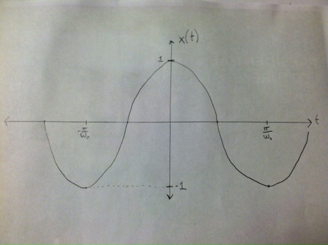
+x(t) = cos(w<sub>o</sub>t) &nbsp; &nbsp;(pictured below)
-<br>
+[[Image:XtEvan.JPG]]
-----
-== Derivation  ==
-Then we are going to find<span style="line-height: 1.5em;">etween </span><span class="texhtml" style="line-height: 1.5em;">''X''<sub>''s''</sub>(''f'')</span><span style="line-height: 1.5em;"> and </span><span class="texhtml" style="line-height: 1.5em;">''X''<sub>''d''</sub>(ω)</span><span style="line-height: 1.5em;"> and the relationship is showed in graph as below:</span>
-<font size="size"><font size="size"><font size="size"><font size="size">
-----
-== example  ==
-<br>
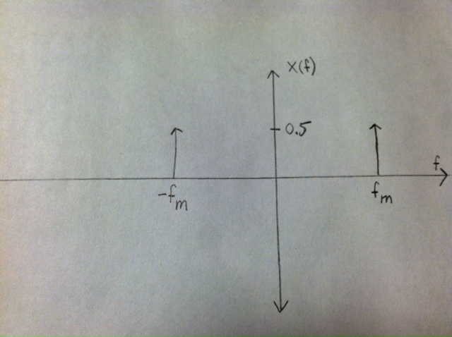
+&nbsp;X(f) = pi*(delta(w-w<sub>o</sub>) + delta(w+w<sub>o</sub>))<br>&nbsp; &nbsp; &nbsp; &nbsp; = 1/2*(delta(f - f<sub>o</sub>) + delta(f + f<sub>o</sub>)) &nbsp; &nbsp; (pictured below)
-fd
+[[Image:Xf.JPG]]<br>
+<br>
+<br>
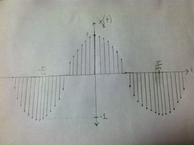
+x<sub>s</sub>(t) = cos(w<sub>o</sub>t) * p<sub>T</sub>(t)<br>&nbsp; &nbsp; &nbsp; &nbsp; = combT(cos(w<sub>o</sub>t)) &nbsp; &nbsp; &nbsp; &nbsp; &nbsp; &nbsp; &nbsp; &nbsp; &nbsp; &nbsp; &nbsp; &nbsp; &nbsp; &nbsp;(pictured below) &nbsp; &nbsp; &nbsp; &nbsp; &nbsp; &nbsp; &nbsp; &nbsp;
+[[Image:XstEvan.JPG]]
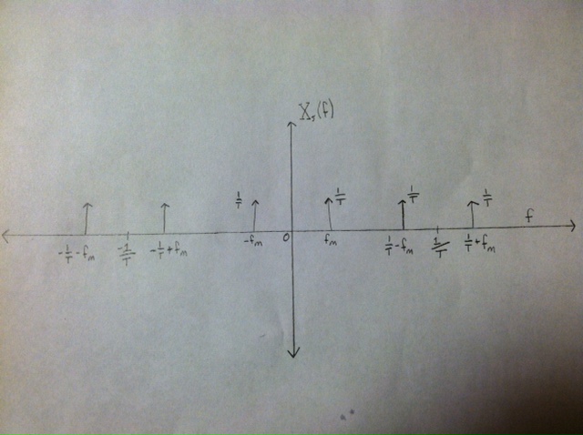
+X<sub>s</sub>(f) = (1/T)*rep1/T(1/2*(delta(f - f<sub>o</sub>) + delta(f + f<sub>o</sub>))) &nbsp; &nbsp; &nbsp; (pictured below)<br>
+[[Image:Xsf.JPG]]
+<br>
+</font></font><font size="size"><font size="size"><font size="size">
 ----
-== conclusion  ==
+== Conclusion  ==
-So t<span class="texhtml">2π''T''</span>
+In conclusion, the frequency domain view of a sampled signal is a scaled and repeated version of the original continuous time signal. The amplitude is scaled by 1/T and the repitition occurs every 1/T.
 ----
-</font></font></font></font></font></font>
+If you have any questions, comments, etc. please post them [[Slecture_Topic_7_Evancomments|right here]].
+</font></font></font>
+<font size="size"><font size="size"><font size="size"></font></font></font>
+<font size="size"><font size="size"><font size="size"></font></font></font>
+<font size="size"><font size="size"><font size="size"></font></font></font>
+<font size="3"><font size="size"><font size="size"><font size="size"></font></font></font></font>
 <font size="3"><font size="size"><font size="size"><font size="size"></font></font></font></font>
 <font size="3"><font size="size"><font size="size"></font> </font> </font>
+----
+[[2014_Fall_ECE_438_Boutin_digital_signal_processing_slectures|Back to ECE438 slectures, Fall 2014]]
 [[Category:Slecture]] [[Category:ECE438Fall2014Boutin]] [[Category:ECE]] [[Category:ECE438]] [[Category:Signal_processing]]