| Line 8: | Line 8: | ||
</center> | </center> | ||
---- | ---- | ||
| + | |||
| + | <font size="3"></font> | ||
<font size="3"></font> | <font size="3"></font> | ||
| Line 39: | Line 41: | ||
The sampling of signal x(t), is the comb of x(t), which is equivalent to multiplying x(t) by the impulse train p<sub>T</sub>(t). | The sampling of signal x(t), is the comb of x(t), which is equivalent to multiplying x(t) by the impulse train p<sub>T</sub>(t). | ||
| − | So, x<sub>s</sub>(t) = x(t) x p<sub>T</sub>(t) = comb<sub>T</sub>(x(t)) | + | So, x<sub>s</sub>(t) = x(t) x p<sub>T</sub>(t) = comb<sub>T</sub>(x(t)) |
| − | F(x<sub>s</sub>(t)) = X<sub>s</sub>(f) = (1/T) * rep<sub>1/T</sub>(X(f)) | + | F(x<sub>s</sub>(t)) = X<sub>s</sub>(f) = (1/T) * rep<sub>1/T</sub>(X(f)) |
| − | Analytically, we can see that the frequency domain view of the sampling's amplitude is scaled by a factor of 1/T. The shape of the frequency responses are the same, but it is repeated every 1/T in the sampling's frequency response. | + | Analytically, we can see that the frequency domain view of the sampling's amplitude is scaled by a factor of 1/T. The shape of the frequency responses are the same, but it is repeated every 1/T in the sampling's frequency response. In the following example we will see the relationship graphically |
<span style="line-height: 1.5em;" /> | <span style="line-height: 1.5em;" /> | ||
| − | <span style="line-height: 1.5em;" /> <font size="size"></font> | + | <span style="line-height: 1.5em;" /> <font size="size"></font> <font size="size"></font> |
<font size="size"> | <font size="size"> | ||
---- | ---- | ||
| Line 53: | Line 55: | ||
== example == | == example == | ||
| − | x(t) = cos(w<sub>o</sub>t) X(f) = pi*(delta(w-w<sub>o</sub>) + delta(w+w<sub>o</sub>))<br> = 1/2*(delta(f - f<sub>o</sub>) + delta(f + f<sub>o</sub>)) | + | x(t) = cos(w<sub>o</sub>t) X(f) = pi*(delta(w-w<sub>o</sub>) + delta(w+w<sub>o</sub>))<br> = 1/2*(delta(f - f<sub>o</sub>) + delta(f + f<sub>o</sub>)) |
| − | x<sub>s</sub>(t) = cos(w<sub>o</sub>t) * p<sub>T</sub>(t) X<sub>s</sub>(f) = (1/T)*rep1/T(1/2*(delta(f - f<sub>o</sub>) + delta(f + f<sub>o</sub>)))<br> = comb<sub>T</sub>(cos(w<sub>o</sub>t)) | + | |
| + | |||
| + | [[Image:Cosine.gif]] | ||
| + | |||
| + | Continuous time plot of x(t) = cos(w<sub>o</sub>t) | ||
| + | |||
| + | |||
| + | |||
| + | |||
| + | |||
| + | x<sub>s</sub>(t) = cos(w<sub>o</sub>t) * p<sub>T</sub>(t) X<sub>s</sub>(f) = (1/T)*rep1/T(1/2*(delta(f - f<sub>o</sub>) + delta(f + f<sub>o</sub>)))<br> = comb<sub>T</sub>(cos(w<sub>o</sub>t)) | ||
<br> | <br> | ||
| Line 64: | Line 76: | ||
</font></font> | </font></font> | ||
| − | <font size="3"> | + | <font size="3"><font size="size"></font></font> |
| − | <font size="3"><span style="line-height: 1.5em;"> </span><span class="texhtml" style="line-height: 1.5em;">''X''<sub>''d''</sub>(ω)</span><span style="line-height: 1.5em;"> and the relationship is showed in graph as below:</span> <font size="size"><font size="size"><font size="size"><font size="size"></font></font></font></font></font> <font size="size"><font size="size"><font size="size"></font></font></font> | + | <font size="3">Then we are going to find<span style="line-height: 1.5em;">etween </span><span class="texhtml" style="line-height: 1.5em;">''X''<sub>''s''</sub>(''f'')</span><span style="line-height: 1.5em;"> and</span></font> |
| + | |||
| + | <font size="3"><span style="line-height: 1.5em;"> </span><span class="texhtml" style="line-height: 1.5em;">''X''<sub>''d''</sub>(ω)</span><span style="line-height: 1.5em;"> and the relationship is showed in graph as below:</span> <font size="size"><font size="size"><font size="size"><font size="size"></font></font></font></font></font> <font size="size"><font size="size"><font size="size"></font></font></font> | ||
| + | |||
| + | <font size="size"><font size="size"><font size="size"></font></font></font> | ||
<font size="size"><font size="size"><font size="size"> | <font size="size"><font size="size"><font size="size"> | ||
| Line 85: | Line 101: | ||
---- | ---- | ||
</font></font></font> | </font></font></font> | ||
| + | |||
| + | <font size="size"><font size="size"><font size="size"></font></font></font> | ||
<font size="size"><font size="size"><font size="size"></font></font></font> | <font size="size"><font size="size"><font size="size"></font></font></font> | ||
Revision as of 19:16, 6 October 2014
Frequency domain view of the relationship between a signal and a sampling of that signal
A slecture by ECE student Evan Stockrahm
Partly based on the ECE438 Fall 2014 lecture material of Prof. Mireille Boutin.
Outline
- Introduction
- Derivation
- Example
- Conclusion
Introduction
This slecture will discuss the frequency domain view of the relationship between a signal, and a sampling of that signal. Essentially, given a signal x(t), we are going to take a look at the similarities and differences in X(f) and Xs(f). Xs(f) is the Fourier Transform of the sampling, xs(t), of x(t).
Derivation
Given an arbitrary signal x(t), its Fourier Transform is X(f)
The sampling of signal x(t), is the comb of x(t), which is equivalent to multiplying x(t) by the impulse train pT(t).
So, xs(t) = x(t) x pT(t) = combT(x(t))
F(xs(t)) = Xs(f) = (1/T) * rep1/T(X(f))
Analytically, we can see that the frequency domain view of the sampling's amplitude is scaled by a factor of 1/T. The shape of the frequency responses are the same, but it is repeated every 1/T in the sampling's frequency response. In the following example we will see the relationship graphically
<span style="line-height: 1.5em;" />
<span style="line-height: 1.5em;" />
example
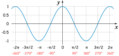
x(t) = cos(wot) X(f) = pi*(delta(w-wo) + delta(w+wo))
= 1/2*(delta(f - fo) + delta(f + fo))
Continuous time plot of x(t) = cos(wot)
xs(t) = cos(wot) * pT(t) Xs(f) = (1/T)*rep1/T(1/2*(delta(f - fo) + delta(f + fo)))
= combT(cos(wot))
Derivation
Then we are going to findetween Xs(f) and
Xd(ω) and the relationship is showed in graph as below:
example
fd
conclusion
So t2πT


