Comment from Prof. Mimi: Since I didn't teach this, you should call this "A supplement to Prof. Mimi ECE662 Course blah blah" rather than "Partly based on Prof. Mimi's course blah blah"

In class, we covered the simple Bayesian classifier. This form of classification falls under a category known as supervised learning. What this means is that a set of labelled data data is used to to "train" the underlying model. However, it is not always possible to have such a data set, yet we may still wish to discover some form of underlying structure in an unlabelled data set. Such a task falls under the category of unsupervised learning.

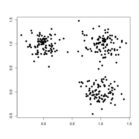
Clustering is a form of unsupervised learning. "Clustering is the problem of identifying groups, or clusters of data points in multidimensional space". For example, consider the following data set:

Figure 1

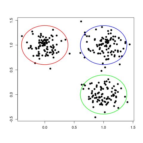
Although this data set is not labelled, we can still clearly see three different groups, or clusters, of data points, as shown here:

Figure 2

In some ways, each cluster can be thought of a different "class" of data points. In this way, clustering can be seen as the unsupervised analog of the classification problem.

There is no "best" clustering algorithm. Any algorithm imposes some sort of structure on the data. If the structure imposed by the clustering algorithm matches the true structure of the data, then the actual clusters may be discovered. As a result, there are many different clustering methods. Here I will describe a popular and intuitive method known as K-means clustering.

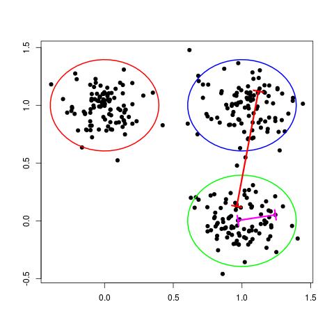
One way of thinking about a cluster is a set of points who's pairwise distances are small compared to the distance to the points of a different cluster. This is illustrated in the following figure:

Figure 3

In the figure above, the magenta line represents a general distance between two points of the same cluster and the red line represents a general distance between points of different clusters. Intuitively, we expect the red line to be significantly longer than the magenta line.

The K-means algorithm formalizes this by first introducing a set of $ D $-dimensional vectors, $ \mu_k $, where $ k = 1,...,K $. These vectors represent the current guess for the center of each cluster. As you will see later, throughout the k-means algorithm, we optimize the locations of these centers and the assignment of data points to specific clusters.

The K-means algorithm also introduces a set of binary variables to represent assignment of data points to specific clusters:
$ r_{nk} \in \{0,1\} $
where $ k = 1,...,K $ and $ n = 1,...,N $ and $ N $ is the total number of data points.
This set of binary variables is interpreted as follows: if data point $ n $ is assigned to cluster $ k $, then $ r_{nk} = 1 $, otherwise $ r_{nk} = 0 $.

Now, given a set of data points $ \{X_1,...,X_N\} $, we can define a cost function:

What this represents is the sum of squares of the distance of each data point to it's assigned vector $ \mu_k $. To see this, notice that since $ r_{nk} = 1 $ only when point $ n $ has been assigned to cluster $ k $, that is the only distance that gets added to our total cost function. All other combinations of $ n $ and $ k $ lead to $ r_{nk} = 0 $, and thus do not affect the total cost function, $ J $.

Back to ECE662, Spring 2014