Nyquist Michael Hayashi ECE438 slecture - Rhea

Statement of Theorem

The Nyquist Theorem states that a signal may be perfectly reconstructed from its sampling provided that the original signal contains no frequency content above or equal to the sampling frequency. Applying mathematical expressions to the theorem, a signal $ x(t) $ may certainly be reconstructed perfectly from its sampling $ x_s(t) $if the continuous-time Fourier Transform (CTFT) of $ x(t) $ is zero for all magnitudes of frequency equal to or above half the sampling frequency (Nyquist condition).

Let the Nyquist sampling rate $ f_s $ be equal to this frequency of interest for reconstruction where $ f_M $ denotes the magnitude of the largest nonzero frequency in $ x(t) $:
$ f_s \triangleq 2f_M $

Nyquist condition:
$ X(f) = 0 \ \forall \ |f| \geq \frac{1}{2T} $

Using the Nyquist condition to set the sampling period $ T $:
$ \frac{1}{T} > 2f_M \ or \ T < \frac{1}{f_s} $

Simple Example: Frequency Domain

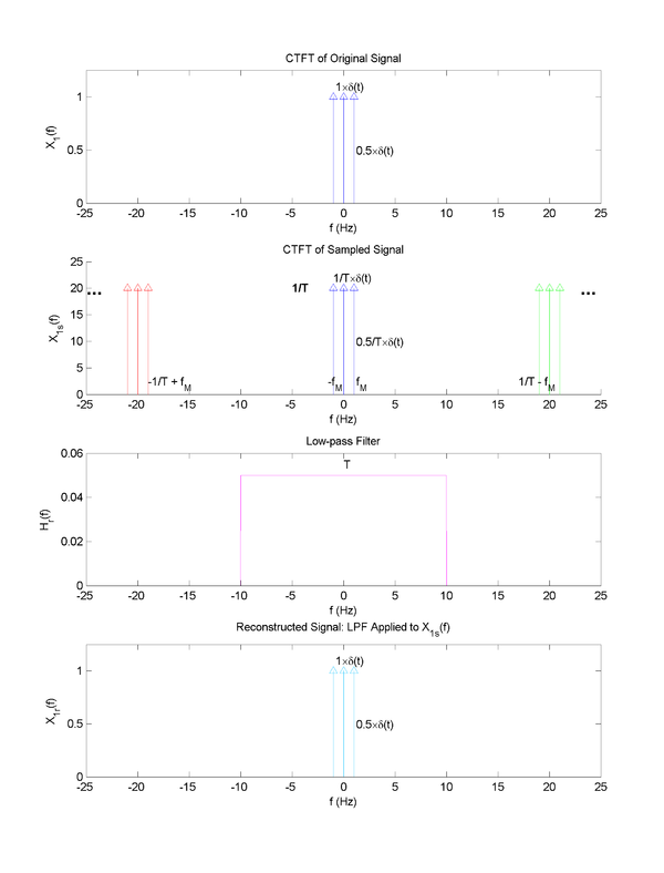
The topmost plot in the figure above shows the continuous-time Fourier Transform (CTFT) of the signal of interest for this example: a 1-Hz cosine wave with a constant offset of 1. The center Dirac delta-function (corresponding to f=0 Hz) has a coefficient of 1 due to the additive constant while the delta-functions on the left and right (corresponding to f=-1 Hz and f=1 Hz) share a coefficient of 0.5.

The middle-top plot shows the CTFT of an ideal sampling of the signal corresponding to multiplication by a comb generator of period $ T $ in the time domain. Note that $ X_{1s}(f) $ is equivalent to $ X_1(f) $ with repetitions every $ T^{-1} = 20 $ and scaled by $ T^{-1} $. In order to have the copies of the original signal be distinct from one another, there must be a non-zero spacing between each one. Allow $ f_M $ to denote the magnitude of the frequency of the cosine wave (the largest frequency present in the original signal) as defined above.

For the gap right of the center copy,
$ \frac{1}{T} - f_M > f_M \ \longrightarrow \ \frac{1}{T} > 2 \times f_m \ \longrightarrow \ \frac{1}{T} > f_s $

The same result proving the Nyquist condition results for the gap left of the center copy,
$ -f_M > \frac{-1}{T} + f_M \ \longrightarrow \ \frac{1}{T} > 2f_m $

The middle-bottom plot shows the ideal low-pass filter (LPF) that can be used to recover the original signal from this sampling. In this case, $ H_r(f) $ has a gain of $ T $ and a cutoff frequency of $ f_{co} = \frac{1}{2T} = 10 \ Hz $.

The bottommost plot shows the results of applying the LPF to the sampling,
$ X_{1r}(f) = H_{r}(f) \times X_{1s}(f) $.
By meeting the Nyquist condition, the reconstructed signal was guaranteed to equal the original signal.

Simple Example: Time Domain and Whitaker-Kotelnikov-Shannon Reconstruction

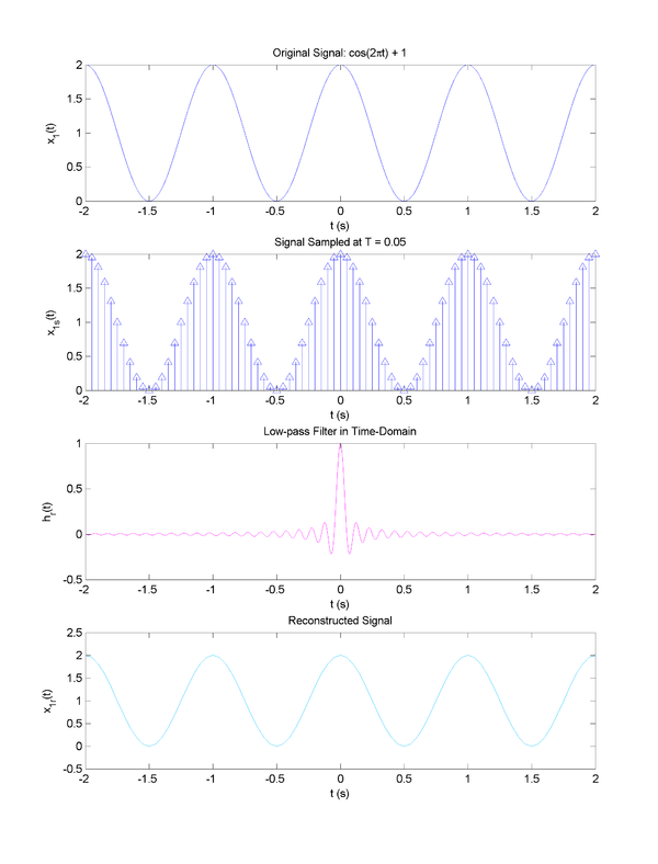
The figure above shows the same signals as in the figure in the previous section except in the time domain. The topmost plot shows the 1-Hz cosine wave with a constant offset of 1 that served as the simple example preceding this section. The middle-top plot shows the combed function of the signal with delta-functions with the coefficients corresponding to the y-values. The sampling rate of $ T^{-1} = 20 $ means that there are 20 samples in every 1-second interval.

The middle-bottom plot shows the time-domain representation of the low-pass filter with gain $ T $ and a cutoff frequency $ f_{co} $ of 10 Hz. Just as the frequency-domain representation was a $ rect() $ function, the time-domain representation is a $ sinc() $ function. The bottom plot shows the reconstructed signal. Because the cascading of the LPF system with the output of the sampling system, the multiplication that occurred in the frequency domain must be a convolution in the time domain. Because of the delta-functions in the sampling, the reconstruction is formed from summing $ sinc() $ functions at the location of each of the infinitely many samples and vertically scaling them by the delta-function coefficient. Even with only four periods worth of samples, the reconstruction is virtually identical to the original signal.

$ H_r(f) = T \times rect(Tf) $

$ h_r(t) = sinc(\frac{t}{T}) $

$ x_r(t) = \sum_{n=-\infty}^{\infty} x(nT) \times sinc(\frac{t - nT}{T}) $

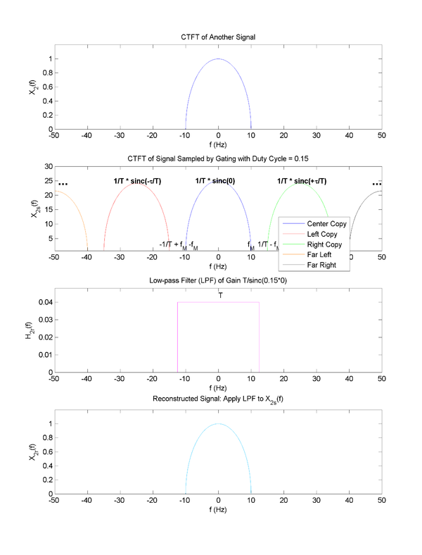
More Complicated Example

---

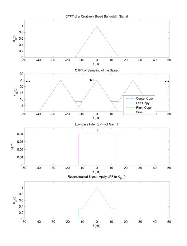
Nyquist Condition Violation Example

Important Notes

1. The Nyquist condition guarantees that the original signal may be reconstructed from the sampling, but there are signals that have CTFT's that allow for perfect reconstruction even when the Nyquist condition is violated.
2. For signals with discontinuous CTFT magnitudes, $ f_s $ may be more clearly defined by stating that the Nyquist sampling rate is the least such frequency magnitude of $ X(f) $ for which $ X(f) = 0 $. This definition firmly places $ f_s $ outside any jumps to $ X(f) = 0 $.
3. Restricting the Nyquist Theorem to purely real signals (the only physically producible signals) that have equal nonzero extent both in the positive-f and negative-f directions, the wording of the Nyquist condition may be relaxed to state that the CTFT of the original signal must not contain any frequencies equal to or higher than half the sampling frequency.

TO BE CONTINUED

Questions and comments

If you have any questions, comments, etc. please post them on this page.

Back to ECE438, Fall 2014