| Line 194: | Line 194: | ||
\phi_{12}\,= p \phi_1 + (1-p)\phi_2 | \phi_{12}\,= p \phi_1 + (1-p)\phi_2 | ||
</math></center> | </math></center> | ||
| − | This test can be implmented by selecting \phi_1 and \phi_2 at random with probability p and 1-p, respectively. The level of this test is | + | This test can be implmented by selecting <math>\phi_1</math> and <math>\phi_2</math> at random with probability p and 1-p, respectively. The level of this test is |
| + | <center><math> | ||
| + | \alpha_{12} = E_0[\phi_{12}] = p E_0[\phi_1] + (1-p)E_0[\phi_2] = p\alpha_1 + (1-p)\alpha_2 | ||
| + | </math></center> | ||
| + | and its power is similarly | ||
| + | <center><math> | ||
| + | \beta_{12} = E_1[\phi_{12}] = p\beta_1 + (1-p)\beta_2 | ||
| + | </math></center> | ||
| + | |||
| + | |||
| + | |||
| + | |||
| + | |||
| + | |||
| + | |||
| + | |||
| + | |||
| + | |||
Revision as of 01:59, 1 May 2014
Neyman-Pearson Lemma and Receiver Operating Characteristic Curve
A slecture by ECE student Soonam Lee
Partly based on the ECE662 Spring 2014 lecture material of Prof. Mireille Boutin.
Contents
INTRODUCTION
The purpose of this slecture is understanding Neyman-Pearson Lemma and Receiver Operating Characteristic (ROC) curve from theory to application. The fundamental theories stem from statistics and these can be used for signal detection and classification. In order to firmly understand these concepts, we will review statistical concept first including False alarm and Miss. After that, we will consider Bayes' decision rule using cost function. Next, we visit Neyman-Pearson test and minimax test. Lastly, we will discuss ROC curves. Note that we only consider two classes case in this slecture, but the concept can be extended to multiple classes.
THE GENERAL TWO CLASSES CASE PROBLEM
Before starting our discussion, we have the following setup:
- $ X $ a measure random variable, random vector, or random process
- $ x \in \mathcal{X} $ is a realization of $ X $
- $ \theta \in \Theta $ are unknown parameters
- $ f(x; \theta) $ is pdf of $ X $ (a known function)
Two distinct hypotheses on $ \theta $ such that $ H_0: \theta \in \Theta_0 $ versus $ H_1: \theta \in \Theta_1 $ where $ \Theta_0 $, $ \Theta_1 $ is partition of $ \Theta $ into two disjoint regions
FALSE ALARM RATE AND MISS RATE
From statistical references [1, 2], these two hypotheses make one of two types of error, named Type I Error and Type II Error. If $ \theta \in \Theta_0 $ but the hypothesis test incorrectly decides to reject $ H_0 $, then the test has made a Type I Error. If, on the other hand, $ \theta \in \Theta_1 $ but the test decides to accept $ H_0 $ a Type II Error has been made. Type I Error is often called false positive error and Type II Error is called false negative error. These two types are depicted in Table 1.
| Decision Accpet $ H_0 $ |
Decision Reject $ H_0 $ |
|
| Truth $ H_0 $ | Correct Decision | Type I Error |
| Truth $ H_1 $ | Type II Error | Correct Decision |
Table 1: Two types of erros in hypothesis testing.
Different from statistical perspective, engineers focus more on false alarm rate and miss errors rate. False alarm rate is the same as Type I Error such that a given condition has been fulfilled, when it actually has not been fulfilled, that is, erroneously a positive effect has been assumed. Miss rate is such that a given condition has not been fulfilled, when it actually has been fulfilled. In general, to compute miss rate, computing hit rate and subtract hit rate from 1 to get miss rate.
Let's assume a test function $ \phi(x) $ such that
| $ \phi(x) = \, $ | $ \, \Big\{ $ |
|
The test function $ \phi(x) $ maps $ \mathcal{X} $ to the decision space $ \{0, 1\} $ for deciding $ H_0 $ and $ H_1 $. The function $ \phi(x) $ induces a partition of $ \mathcal{X} $ into decision regions. Denote $ \mathcal{X}_0 = \{x: \phi(x) = 0 \} $ and $ \mathcal{X}_1 = \{x: \phi(x) = 1 \} $. Then, false alarm and miss probabilities with the function $ \phi $ can be expressed as follow:
The probability of correctly deciding $ H_1 $ is called hit probability such that
From the ECE 662 class note [3], Professor Boutin introduced error 1 ($ \epsilon_1 $) and error 2 ($ \epsilon_2 $) that are basically same concepts as miss rate and false alarm rate respectively. The only difference is representing the expectation values as fraction as follow:
NEYMAN-PEARSON LEMMA [4, 5]
The frequentist approach assumes no priors on $ H_0 $ or $ H_1 $ so one cannot sensibly define an average probability of error of risk to minimize. Thus we adopt the alternative criterion: constrain false alarm and minimize miss probabilities. It turns out that to find an optimum test satisfying such a constraint we will need to extend our previous definition of a test function $ \phi $ to allow for randomized decisions such that
| $ \phi(x)= \, $ | { |
|
Note, we have interpretation:
False alarm probability and detection probability are functions of $ \theta $
| $ E_\theta [\phi] = \int_{\mathcal{X}} \phi(x) f(x; \theta) dx = $ | { |
|
We define a test $ \phi $ is said to be (false alarm) level $ \alpha \in [0,1] $ if
We also define the power function of a test $ \phi $ as
Here, we consider only simple hypotheses case where $ \theta \in \{\theta_0, \theta_1\} $
Then, we will introduce the Neyman-Pearson strategy such that find the most powerful (MP) test $ \phi^* $ of level $ \alpha $:
for any other test satisfying $ E_{\theta_0} [\phi] \leq \alpha. $ Note that Neyman-Pearson Lemma is defined as the MP test of level $ \alpha \in [0,1] $ is a randomized likelihood ratio test (LRT) of the form
| $ \phi(x)^* = \, $ | { |
|
where $ \eta $ and $ q $ are selected to satisfy $ E_{\theta_0} [\phi^*] = \alpha. $ Let's denote this LRT as $ \Lambda(x) $. Then, the shorthand LRT notation will be
ROC CURVES FOR THRESHOLD TESTS [5]
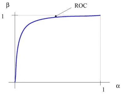
From this section, we will look through the definition of ROC curve and the properties of ROC curve. All threshold tests have $ P_F $ and $ P_D $ indexed by a parameter $ \eta $. The Receiver Operating Characteristic (ROC) is simply the plot of the parameteric curve $ \{P_F(\eta, q), P_D(\eta, q)\}_\eta.\, $ Equivalently, ROC is the plot of $ \beta = P_D\, $ versus $ \alpha = P_F\, $. A typical ROC curve using these $ \alpha $ and $ \beta $ is shown in Figure 1.
Figure 1: A typical ROC curve.
This ROC curve has several properties as follow:
- ROC for coin flip detector ($ \phi(x) = q $ independent of data) is a diaognal line with slope = 1. Since this coin flip produces fifty-fifty chances of each output, the chance line is diagonal in ROC curve. Figure 2 is the result for coin flip detector.
Figure 2: ROC curve for coin flip detector.
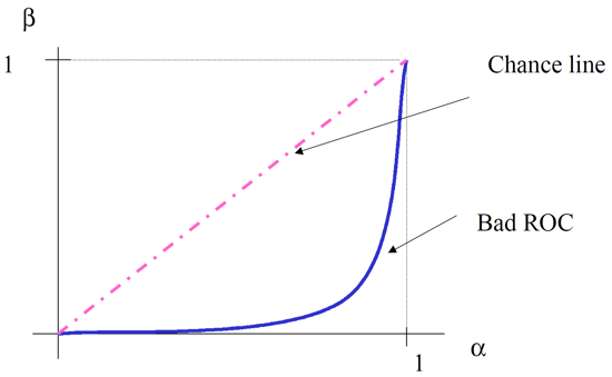
- ROC of any MP test always lies above diagonal. MP test is unbiased test. A test $ \phi $ is unbiased if its detection probability $ \beta $ is at least as great as its false alarm $ \alpha $: $ \beta > \alpha. $ The bad ROC example is shown in Figure 3. As you can see from the figure, good ROC curve should be always above the diagonal.
Figure 3: ROC curve for MP test always lines above diagonal.
- ROC of any MP test is always convex cap (concave). To see concavity, let ($ \alpha_1 $, $ \beta_1 $) be the level and power of a test $ \phi_1 $ and ($ \alpha_2 $, $ \beta_2 $) be the level and power of a test $ \phi_2 $. Define the test
This test can be implmented by selecting $ \phi_1 $ and $ \phi_2 $ at random with probability p and 1-p, respectively. The level of this test is
and its power is similarly
REFERENCES
[1] G. Casella and R. L. Berger, "Statistical inference (2nd Edition)," Cengage Learning, 2001.
[2] J. K. Ghosh, "STAT528: Introduction to Mathematical Statistics," Fall 2012, Purdue University.
[3] M. Boutin, "ECE662: Statistical Pattern Recognition and Decision Making Process," Spring 2014, Purdue University.
[4] K. Fukunaga, "Introduction to statistical pattern recognition (2nd Edition)," Academic Press, Inc., San Diego, CA, USA, 1990.
[5] A. Hero, "EECS564: Esitmation, Filtering, and Detection," Fall 2010, University of Michigan.
Questions and comments
If you have any questions, comments, etc. please post them on this page.


