(→Lecture Objective) |
|||
| (14 intermediate revisions by 3 users not shown) | |||
| Line 1: | Line 1: | ||
| − | [ | + | =Lecture 8, [[ECE662]]: Decision Theory= |
| − | [ | + | Lecture notes for [[ECE662:BoutinSpring08_Old_Kiwi|ECE662 Spring 2008]], Prof. [[user:mboutin|Boutin]]. |
| + | |||
| + | Other lectures: [[Lecture 1 - Introduction_Old Kiwi|1]], | ||
| + | [[Lecture 2 - Decision Hypersurfaces_Old Kiwi|2]], | ||
| + | [[Lecture 3 - Bayes classification_Old Kiwi|3]], | ||
| + | [[Lecture 4 - Bayes Classification_Old Kiwi|4]], | ||
| + | [[Lecture 5 - Discriminant Functions_Old Kiwi|5]], | ||
| + | [[Lecture 6 - Discriminant Functions_Old Kiwi|6]], | ||
| + | [[Lecture 7 - MLE and BPE_Old Kiwi|7]], | ||
| + | [[Lecture 8 - MLE, BPE and Linear Discriminant Functions_Old Kiwi|8]], | ||
| + | [[Lecture 9 - Linear Discriminant Functions_Old Kiwi|9]], | ||
| + | [[Lecture 10 - Batch Perceptron and Fisher Linear Discriminant_Old Kiwi|10]], | ||
| + | [[Lecture 11 - Fischer's Linear Discriminant again_Old Kiwi|11]], | ||
| + | [[Lecture 12 - Support Vector Machine and Quadratic Optimization Problem_Old Kiwi|12]], | ||
| + | [[Lecture 13 - Kernel function for SVMs and ANNs introduction_Old Kiwi|13]], | ||
| + | [[Lecture 14 - ANNs, Non-parametric Density Estimation (Parzen Window)_Old Kiwi|14]], | ||
| + | [[Lecture 15 - Parzen Window Method_Old Kiwi|15]], | ||
| + | [[Lecture 16 - Parzen Window Method and K-nearest Neighbor Density Estimate_Old Kiwi|16]], | ||
| + | [[Lecture 17 - Nearest Neighbors Clarification Rule and Metrics_Old Kiwi|17]], | ||
| + | [[Lecture 18 - Nearest Neighbors Clarification Rule and Metrics(Continued)_Old Kiwi|18]], | ||
| + | [[Lecture 19 - Nearest Neighbor Error Rates_Old Kiwi|19]], | ||
| + | [[Lecture 20 - Density Estimation using Series Expansion and Decision Trees_Old Kiwi|20]], | ||
| + | [[Lecture 21 - Decision Trees(Continued)_Old Kiwi|21]], | ||
| + | [[Lecture 22 - Decision Trees and Clustering_Old Kiwi|22]], | ||
| + | [[Lecture 23 - Spanning Trees_Old Kiwi|23]], | ||
| + | [[Lecture 24 - Clustering and Hierarchical Clustering_Old Kiwi|24]], | ||
| + | [[Lecture 25 - Clustering Algorithms_Old Kiwi|25]], | ||
| + | [[Lecture 26 - Statistical Clustering Methods_Old Kiwi|26]], | ||
| + | [[Lecture 27 - Clustering by finding valleys of densities_Old Kiwi|27]], | ||
| + | [[Lecture 28 - Final lecture_Old Kiwi|28]], | ||
| + | ---- | ||
| + | ---- | ||
| + | |||
| + | |||
| + | __TOC__ | ||
== Lecture Objective == | == Lecture Objective == | ||
| Line 10: | Line 44: | ||
[[Image:MLEvBPE comparison_Old Kiwi.jpg]] | [[Image:MLEvBPE comparison_Old Kiwi.jpg]] | ||
| − | If the prior distributions have some specific properties | + | If the prior distributions have some specific properties then the Bayesian Parameter Estimation and Maximum Likelihood Estimation are asymptotically equivalent for infinite training data. However, large training datasets are typically unavailable in pattern recognition problems. Furthermore, when the dimension of data increases, the complexity of estimating the parameters increases exponentially. In that aspect, BPE and MLE have some advantages over each other. |
*Computational Complexity: | *Computational Complexity: | ||
| Line 20: | Line 54: | ||
*Form of Distribution: | *Form of Distribution: | ||
The advantage of using BPE is that it uses prior information that we have about the model and it gives us a possibility to sequentially update the model. If the information we have on the model is reliable than BPE is better than MLE. On the other hand, if prior model is uniformly distributed than BPE is not so different than MLE. Indeed, MLE is a special and simplistic form of BPE. | The advantage of using BPE is that it uses prior information that we have about the model and it gives us a possibility to sequentially update the model. If the information we have on the model is reliable than BPE is better than MLE. On the other hand, if prior model is uniformly distributed than BPE is not so different than MLE. Indeed, MLE is a special and simplistic form of BPE. | ||
| − | |||
| − | |||
Figure for BPE processes: | Figure for BPE processes: | ||
[[Image:BPEprocess_Old Kiwi.jpg]] | [[Image:BPEprocess_Old Kiwi.jpg]] | ||
| + | |||
| + | See also: [[Comparison of MLE and Bayesian Parameter Estimation_Old Kiwi]] | ||
| + | |||
| + | == Linear Discriminant Functions == | ||
| + | (From [["Pattern Classification" by Duda, Hart, and Stork_Old Kiwi|DHS]] Chapter 5) | ||
| + | |||
| + | [[Image:Lec8LDF_Old Kiwi.jpg]] | ||
| + | |||
| + | Suppose we have <math>p(w_1|\vec{x})</math> and <math>p(w_2|\vec{x})</math> | ||
| + | |||
| + | <math>g(\vec{x}) = p(w_1|\vec{x}) - p(w_2|\vec{x}) </math> | ||
| + | |||
| + | <math>p(\vec{x}|w_i)</math> -> Parametric Estimation Method | ||
| + | |||
| + | <math>g(\vec{x})</math> -> proper form of Linear Discriminant Function | ||
| + | |||
| + | <math>[1,x,x^2,x^3] </math> -> new feature space | ||
| + | |||
| + | Simple and easy to design: | ||
| + | |||
| + | *1 category case: | ||
| + | |||
| + | [[Image:Lec8_1_Old Kiwi.jpg]] | ||
| + | |||
| + | <math>g(\vec{x}) = w\vec{x} + w_0</math> | ||
| + | |||
| + | where <math>w</math> is the weight factor and <math>w_0</math> is the bias of the threshold | ||
| + | |||
| + | *2 category case: | ||
| + | |||
| + | <math>w_1, g(\vec{x}) > 0</math> | ||
| + | |||
| + | <math>w_2, g(\vec{x}) < 0</math> | ||
| + | |||
| + | <math>g(\vec{x}) = 0</math> : decision surface | ||
| + | |||
| + | [[Image:Lec8_2_Old Kiwi.jpg]] | ||
| + | |||
| + | <math>g(\vec{x_1}) = w'\vec{x_1} + w_0</math> | ||
| + | |||
| + | <math>g(\vec{x_2}) = w'\vec{x_2} + w_0</math> | ||
| + | |||
| + | <math>w'\vec{x_1} + w_0 = w'\vec{x_2} + w_0</math> | ||
| + | |||
| + | <math>w'(\vec{x_1} - \vec{x_2}) = 0</math> | ||
| + | |||
| + | *N category case: | ||
| + | |||
| + | [[Image:Lec8_3_Old Kiwi.jpg]] | ||
| + | |||
| + | <math>\vec{x} = \vec{x_p} + r\frac{\vec{w}}{|\vec{w}|}</math> | ||
| + | |||
| + | where <math>\vec{x_p}</math> is the projection point, <math>r</math> is the distance, and <math>\frac{\vec{w}}{|\vec{w}|}</math> is the unit normal | ||
| + | |||
| + | <math>g(\vec{x}) = w'\vec{x} + w_0 = w'(\vec{x_p} + r\frac{\vec{w}}{|\vec{w}|}) + w_0 = w'\vec{x_p} + w_0 + w'r\frac{\vec{w}}{|\vec{w}|} = r|\vec{w}|</math> | ||
| + | |||
| + | therefore <math>r = \frac{g(\vec{x})}{|\vec{w}|}</math> | ||
| + | |||
| + | '''For more information:''' | ||
| + | |||
| + | [[Parametric Estimators_Old Kiwi]] | ||
| + | |||
| + | [[Category:Lecture Notes]] | ||
Latest revision as of 08:48, 17 January 2013
Lecture 8, ECE662: Decision Theory
Lecture notes for ECE662 Spring 2008, Prof. Boutin.
Other lectures: 1, 2, 3, 4, 5, 6, 7, 8, 9, 10, 11, 12, 13, 14, 15, 16, 17, 18, 19, 20, 21, 22, 23, 24, 25, 26, 27, 28,
Contents
Lecture Objective
- Maximum Likelihood Estimation and Bayesian Parameter Estimation
- Linear Discriminant Functions
Maximum Likelihood Estimation and Bayesian Parameter Estimation
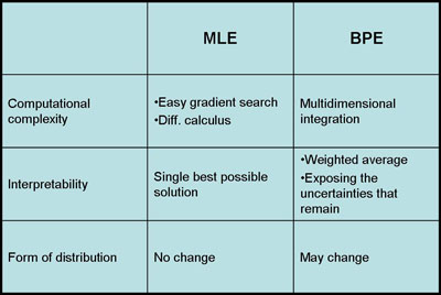
If the prior distributions have some specific properties then the Bayesian Parameter Estimation and Maximum Likelihood Estimation are asymptotically equivalent for infinite training data. However, large training datasets are typically unavailable in pattern recognition problems. Furthermore, when the dimension of data increases, the complexity of estimating the parameters increases exponentially. In that aspect, BPE and MLE have some advantages over each other.
- Computational Complexity:
MLE has a better performance than BPE for large data, because MLE simply uses gradient or differential calculus to estimate the parameters. On the other hand, BPE uses high dimensional integration and it's computationally expensive.
- Interpretability:
The results of MLE are easier to interpret because it generates a single model to fit the data as much as possible. However, BPE generates a weighted sum of models which is harder to understand.
- Form of Distribution:
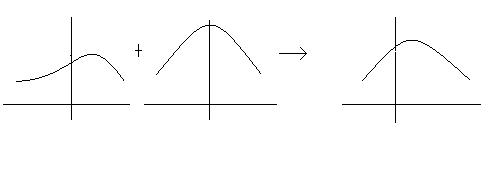
The advantage of using BPE is that it uses prior information that we have about the model and it gives us a possibility to sequentially update the model. If the information we have on the model is reliable than BPE is better than MLE. On the other hand, if prior model is uniformly distributed than BPE is not so different than MLE. Indeed, MLE is a special and simplistic form of BPE.
See also: Comparison of MLE and Bayesian Parameter Estimation_Old Kiwi
Linear Discriminant Functions
(From DHS Chapter 5)
Suppose we have $ p(w_1|\vec{x}) $ and $ p(w_2|\vec{x}) $
$ g(\vec{x}) = p(w_1|\vec{x}) - p(w_2|\vec{x}) $
$ p(\vec{x}|w_i) $ -> Parametric Estimation Method
$ g(\vec{x}) $ -> proper form of Linear Discriminant Function
$ [1,x,x^2,x^3] $ -> new feature space
Simple and easy to design:
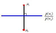
- 1 category case:
$ g(\vec{x}) = w\vec{x} + w_0 $
where $ w $ is the weight factor and $ w_0 $ is the bias of the threshold
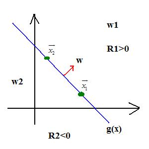
- 2 category case:
$ w_1, g(\vec{x}) > 0 $
$ w_2, g(\vec{x}) < 0 $
$ g(\vec{x}) = 0 $ : decision surface
$ g(\vec{x_1}) = w'\vec{x_1} + w_0 $
$ g(\vec{x_2}) = w'\vec{x_2} + w_0 $
$ w'\vec{x_1} + w_0 = w'\vec{x_2} + w_0 $
$ w'(\vec{x_1} - \vec{x_2}) = 0 $
- N category case:
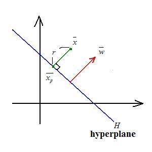
$ \vec{x} = \vec{x_p} + r\frac{\vec{w}}{|\vec{w}|} $
where $ \vec{x_p} $ is the projection point, $ r $ is the distance, and $ \frac{\vec{w}}{|\vec{w}|} $ is the unit normal
$ g(\vec{x}) = w'\vec{x} + w_0 = w'(\vec{x_p} + r\frac{\vec{w}}{|\vec{w}|}) + w_0 = w'\vec{x_p} + w_0 + w'r\frac{\vec{w}}{|\vec{w}|} = r|\vec{w}| $
therefore $ r = \frac{g(\vec{x})}{|\vec{w}|} $
For more information:

