| Line 78: | Line 78: | ||
p(X|w) is normal for all i. | p(X|w) is normal for all i. | ||
| − | Eg: Length of hair among men is a normal random variable. Same for hairlength in women. | + | Eg: Length of hair among men is a normal random variable. Same for hairlength in women. Now we have: |
| − | Now we have: | + | |
| + | |||
| + | [[Image: Lc5_ellipse_OldKiwi.jpg]] | ||
Revision as of 16:24, 10 March 2008
LECTURE THEME : - Discriminant Functions
Discriminant Functions: one way of representing classifiers
Given the classes $ \omega_1, \cdots, \omega_k $
The discriminant functions $ g_1(x),\ldots, g_K(x) $ such that $ g_i(x) $ n-dim S space $ \rightarrow \Re $
which are used to make decisions as follows:
decide $ \omega_i $ if $ g_i(x) \ge g_j(x), \forall j $
Note that many different choices of $ g_i(x) $ will yield the same decision rule, because we are interested in the order of values of $ g_i(x) $ for each x, and not their exact values.
For example: $ g_i(x) \rightarrow 2(g_i(x)) $ or $ g_i(x) \rightarrow ln(g_i(x)) $
In other words, we can take $ g_i(x) \rightarrow f(g_i(x)) $ for any monotonically increasing function f.
Relation to Bayes Rule
e.g. We can take $ g_i(\mathbf(x)) = P(\omega_i|\mathbf(x)) $
then $ g_i(\mathbf(x)) > g_j(\mathbf(x)), \forall j \neq i $
$ \Longleftrightarrow P(w_i|\mathbf(X)) > P(w_j|\mathbf(X)), \forall j \neq i $
OR we can take
$ g_i(\mathbf(x)) = p(\mathbf(x)|\omega_i)P(\omega_i) $
then $ g_i(\mathbf(x)) > g_j(\mathbf(x)), \forall j \neq i $
$ \Longleftrightarrow g_i(\mathbf(x)) = ln(p(\mathbf(x)|\omega_i)P(\omega_i)) = ln(p(\mathbf(x)|\omega_i))+ln(P(\omega_i) $
OR we can take
$ g_i(\mathbf(x)) = ln(p(\mathbf(x)|\omega_i)P(\omega_i)) = ln(p(\mathbf(x)|\omega_i))+ln(P(\omega_i) $
We can take any $ g_i $ as long as they have the same ordering in value as specified by Bayes rule.
Some useful links:
- Bayes Rule in notes: https://engineering.purdue.edu/people/mireille.boutin.1/ECE301kiwi/Lecture4
- Bayesian Inference: http://en.wikipedia.org/wiki/Bayesian_inference
Relational Decision Boundary
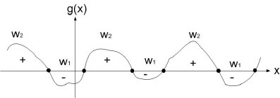
Ex : take two classes $ \omega_1 $ and $ \omega_2 $
$ g(\vec x)=g_1(\vec x)-g_2(\vec x) $
decide $ \omega_1 $ when $ g(\vec x)>0 $
and $ \omega_2 $ when $ g(\vec x)<0 $
when $ g(\vec x) = 0 $, you are at the decision boundary ( = hyperplane)
$ \lbrace \vec x | \vec x \;\;s.t \;\;g(\vec x)=0\rbrace $ is a hypersurface in your feature space i.e a structure of co-dimension one less dimension than space in which $ \vec x $ lies
Discriminant function for the Normal Density
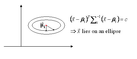
Suppose we assume that the distribution of the feature vectors is such that the density function p(X|w) is normal for all i.
Eg: Length of hair among men is a normal random variable. Same for hairlength in women. Now we have:


