| (45 intermediate revisions by 8 users not shown) | |||
| Line 1: | Line 1: | ||
| − | + | =Lecture 23, [[ECE662]]: Decision Theory= | |
| − | + | Lecture notes for [[ECE662:BoutinSpring08_Old_Kiwi|ECE662 Spring 2008]], Prof. [[user:mboutin|Boutin]]. | |
| − | + | Other lectures: [[Lecture 1 - Introduction_Old Kiwi|1]], | |
| + | [[Lecture 2 - Decision Hypersurfaces_Old Kiwi|2]], | ||
| + | [[Lecture 3 - Bayes classification_Old Kiwi|3]], | ||
| + | [[Lecture 4 - Bayes Classification_Old Kiwi|4]], | ||
| + | [[Lecture 5 - Discriminant Functions_Old Kiwi|5]], | ||
| + | [[Lecture 6 - Discriminant Functions_Old Kiwi|6]], | ||
| + | [[Lecture 7 - MLE and BPE_Old Kiwi|7]], | ||
| + | [[Lecture 8 - MLE, BPE and Linear Discriminant Functions_Old Kiwi|8]], | ||
| + | [[Lecture 9 - Linear Discriminant Functions_Old Kiwi|9]], | ||
| + | [[Lecture 10 - Batch Perceptron and Fisher Linear Discriminant_Old Kiwi|10]], | ||
| + | [[Lecture 11 - Fischer's Linear Discriminant again_Old Kiwi|11]], | ||
| + | [[Lecture 12 - Support Vector Machine and Quadratic Optimization Problem_Old Kiwi|12]], | ||
| + | [[Lecture 13 - Kernel function for SVMs and ANNs introduction_Old Kiwi|13]], | ||
| + | [[Lecture 14 - ANNs, Non-parametric Density Estimation (Parzen Window)_Old Kiwi|14]], | ||
| + | [[Lecture 15 - Parzen Window Method_Old Kiwi|15]], | ||
| + | [[Lecture 16 - Parzen Window Method and K-nearest Neighbor Density Estimate_Old Kiwi|16]], | ||
| + | [[Lecture 17 - Nearest Neighbors Clarification Rule and Metrics_Old Kiwi|17]], | ||
| + | [[Lecture 18 - Nearest Neighbors Clarification Rule and Metrics(Continued)_Old Kiwi|18]], | ||
| + | [[Lecture 19 - Nearest Neighbor Error Rates_Old Kiwi|19]], | ||
| + | [[Lecture 20 - Density Estimation using Series Expansion and Decision Trees_Old Kiwi|20]], | ||
| + | [[Lecture 21 - Decision Trees(Continued)_Old Kiwi|21]], | ||
| + | [[Lecture 22 - Decision Trees and Clustering_Old Kiwi|22]], | ||
| + | [[Lecture 23 - Spanning Trees_Old Kiwi|23]], | ||
| + | [[Lecture 24 - Clustering and Hierarchical Clustering_Old Kiwi|24]], | ||
| + | [[Lecture 25 - Clustering Algorithms_Old Kiwi|25]], | ||
| + | [[Lecture 26 - Statistical Clustering Methods_Old Kiwi|26]], | ||
| + | [[Lecture 27 - Clustering by finding valleys of densities_Old Kiwi|27]], | ||
| + | [[Lecture 28 - Final lecture_Old Kiwi|28]], | ||
| + | ---- | ||
| + | ---- | ||
| − | + | ==Clustering Method, given the pairwise distances== | |
| − | + | Let d be the number of objects. Let <math>DIST_{ij}</math> denote the distance between objects <math>X_i</math> and <math>X_j</math>. The notion of distance here is not clear unless the application itself is considered. For example, when dealing with some psychological studies data, we may have to consult the psychologist himself as to what is the "distance" between given two concepts. These distances form the input to our clustering algorithm. | |
| − | + | The constraint on these distances is that they be | |
| − | edge weights represents distances. | + | - symmetric between any two objects (<math>DIST_{ij}=DIST_{ji}</math>) |
| + | |||
| + | - always positive (<math>DIST_{ij}>=0</math>) | ||
| + | |||
| + | - zero for distance of an object from itself (<math>DIST_{ii}=0</math>) | ||
| + | |||
| + | - follow <math>\bigtriangleup</math> inequality | ||
| + | |||
| + | [[Image:Dist_table_Old Kiwi.jpg]] Table 1 | ||
| + | |||
| + | ''Idea:'' | ||
| + | |||
| + | If <math>DIST_{ij}</math> small => <math>X_i</math>, <math>X_j</math> in same cluster. | ||
| + | |||
| + | If <math>DIST_{ij}</math> large => <math>X_i</math>, <math>X_j</math> in different clusters. | ||
| + | |||
| + | *How to define small or large? One option is to fix a threshold <math>t_0</math>. | ||
| + | |||
| + | such that | ||
| + | |||
| + | <math>t_0</math> < "typical" distance between clusters, and | ||
| + | |||
| + | <math>t_0</math> > "typical" distance within clusters. | ||
| + | |||
| + | Consider the following situation of objects distribution. This is a very conducive situation, and almost any clustering method will work well. | ||
| + | |||
| + | [[Image:ideal_situation_Old Kiwi.jpg]] Figure 1 | ||
| + | |||
| + | |||
| + | A problem arises when thew following situation arises: | ||
| + | |||
| + | [[Image:elongated_cluster_Old Kiwi.jpg]] Figure 2 | ||
| + | |||
| + | Although we see two separate clusters with a thin distribution of objects in between, the algorithm mentioned above identifies only one cluster. | ||
| + | |||
| + | |||
| + | ==Graph Theory Clustering== | ||
| + | |||
| + | dataset <math>\{x_1, x_2, \dots , x_d\}</math> no feature vector given. | ||
| + | |||
| + | given <math>dist(x_i , x_j)</math> | ||
| + | |||
| + | Construct a graph: | ||
| + | * node represents the objects. | ||
| + | * edges are relations between objects. | ||
| + | * edge weights represents distances. | ||
Definitions: | Definitions: | ||
| − | * A ''complete graph'' is a graph with d(d-1)/2 edges. | + | * A ''complete graph'' is a graph with <math>d(d-1)/2</math> edges. |
| − | + | Example: | |
| + | Number of nodes d = 4 | ||
| + | Number of edges e = 6 | ||
| + | [[Image:ECE662_lect23_Old Kiwi.gif]] Figure 3 | ||
| − | * A ''path'' in a graph between | + | [[Image:Kiwi_lec_edges_figure_Old Kiwi.PNG]] Figure 4 |
| + | |||
| + | * A ''subgraph'' <math>G'</math> of a graph <math>G=(V,E,f)</math> is a graph <math>(V',E',f')</math> such that <math>V'\subset V</math> <math>E'\subset E</math> <math>f'\subset f</math> restricted to <math>E'</math> | ||
| + | |||
| + | * A ''path'' in a graph between <math>V_i,V_k \subset V_k</math> is an alternating sequence of vertices and edges containing no repeated edges and no repeated vertices and for which <math>e_i</math> is incident to <math>V_i</math> and <math>V_{i+1}</math>, for each <math>i=1,2,\dots,k-1</math>. (<math>V_1 e_1 V_2 e_2 V_3 \dots V_{k-1} e_{k-1} V_k</math>) | ||
* A graph is "''connected''" if a path exists between any two vertices in the graph | * A graph is "''connected''" if a path exists between any two vertices in the graph | ||
| Line 26: | Line 107: | ||
* A ''component'' is a maximal connected graph. (i.e. includes as many nodes as possible) | * A ''component'' is a maximal connected graph. (i.e. includes as many nodes as possible) | ||
| − | * A ''maximal complete subgraph'' of a graph G is a complete subgraph of G that is not a proper subgraph of any other complete subgraph of G. | + | * A ''maximal complete subgraph'' of a graph <math>G</math> is a complete subgraph of <math>G</math> that is not a proper subgraph of any other complete subgraph of <math>G</math>. |
| − | * A ''cycle'' is a path of non-trivial length k that comes back to the node where it started | + | * A ''cycle'' is a path of non-trivial length <math>k</math> that comes back to the node where it started |
* A ''tree'' is a connected graph with no cycles. The weight of a tree is the sum of all edge weights in the tree. | * A ''tree'' is a connected graph with no cycles. The weight of a tree is the sum of all edge weights in the tree. | ||
| Line 34: | Line 115: | ||
* A ''spanning tree'' is a tree containing all vertices of a graph. | * A ''spanning tree'' is a tree containing all vertices of a graph. | ||
| − | * A ''minimum spanning tree'' (MST) of a graph G is tree having minimal weight among all spanning trees of G. | + | * A ''minimum spanning tree'' (MST) of a graph G is tree having minimal weight among all spanning trees of <math>G</math>. |
| + | |||
| + | |||
| + | (There are more terminologies for graph theory [http://en.wikipedia.org/wiki/Glossary_of_graph_theory here] ) | ||
| + | |||
| + | Illustration [[Image:Spark1_Old Kiwi.jpg]] Figure 5 | ||
| + | |||
| + | |||
| + | [[Image:Spark2_Old Kiwi.jpg]] Figure 6 | ||
| + | This is spanning tree (MST with weight 4) | ||
| + | |||
| + | [[Image:Spark3_Old Kiwi.jpg]] Figure 7 | ||
| + | Another spanning tree (Also, MST with weight 4) | ||
| + | |||
| + | [[Image:Spark4_Old Kiwi.jpg]] Figure 8 | ||
| + | Not spannning tree (Include 'cycle') | ||
| + | |||
| + | [[Image:Spark5_Old Kiwi.jpg]] Figure 9 | ||
| + | Not spanning tree (No edge for 4) | ||
| + | |||
| + | |||
| + | |||
| + | |||
| + | ---- | ||
| + | |||
| + | ==Graphical Clustering Methods== | ||
| + | |||
| + | * "Similarity Graph Methods" | ||
| + | |||
| + | Choose distance threshold <math>t_0</math> | ||
| + | |||
| + | If <math>dis(X_i,X_j)<t_0</math> draw an ege between <math>X_i</math> and <math>X_j</math> | ||
| + | |||
| + | |||
| + | |||
| + | Example) <math>t_0= 1.3</math> | ||
| + | |||
| + | [[Image:Fig2_1_Old Kiwi.jpg]] | ||
| + | Fig 3-1 | ||
| + | |||
| + | Can define clusters as the connected component of the similarity graph | ||
| + | |||
| + | => Same result as "Single linkage algorithms" | ||
| + | |||
| + | <math>X_i \sim X_j</math> if there is chain | ||
| + | |||
| + | <math>X_i \sim X_{i_1} \sim X_{i_2} \sim \cdots X_{i_k} \sim X_{j}</math> complete | ||
| + | |||
| + | Can also define clusters as the maximal subgraphs of similarity graph | ||
| + | |||
| + | [[Image:Fig2_2_Old Kiwi.jpg]] | ||
| + | Fig 3-2 | ||
| + | |||
| + | =>this yeilds more compact, less enlongated clusters | ||
| + | |||
| + | The approach above is not good for, say, | ||
| + | |||
| + | [[Image:Fig3_3_Old Kiwi.jpg]] | ||
| + | Fig 3-3 | ||
| + | |||
| + | [[Category:Lecture Notes]] | ||
Latest revision as of 08:43, 17 January 2013
Contents
Lecture 23, ECE662: Decision Theory
Lecture notes for ECE662 Spring 2008, Prof. Boutin.
Other lectures: 1, 2, 3, 4, 5, 6, 7, 8, 9, 10, 11, 12, 13, 14, 15, 16, 17, 18, 19, 20, 21, 22, 23, 24, 25, 26, 27, 28,
Clustering Method, given the pairwise distances
Let d be the number of objects. Let $ DIST_{ij} $ denote the distance between objects $ X_i $ and $ X_j $. The notion of distance here is not clear unless the application itself is considered. For example, when dealing with some psychological studies data, we may have to consult the psychologist himself as to what is the "distance" between given two concepts. These distances form the input to our clustering algorithm.
The constraint on these distances is that they be
- symmetric between any two objects ($ DIST_{ij}=DIST_{ji} $)
- always positive ($ DIST_{ij}>=0 $)
- zero for distance of an object from itself ($ DIST_{ii}=0 $)
- follow $ \bigtriangleup $ inequality
 Table 1
Idea:
If $ DIST_{ij} $ small => $ X_i $, $ X_j $ in same cluster.
If $ DIST_{ij} $ large => $ X_i $, $ X_j $ in different clusters.
- How to define small or large? One option is to fix a threshold $ t_0 $.
such that
$ t_0 $ < "typical" distance between clusters, and
$ t_0 $ > "typical" distance within clusters.
Consider the following situation of objects distribution. This is a very conducive situation, and almost any clustering method will work well.
 Figure 1
A problem arises when thew following situation arises:
 Figure 2
Although we see two separate clusters with a thin distribution of objects in between, the algorithm mentioned above identifies only one cluster.
Graph Theory Clustering
dataset $ \{x_1, x_2, \dots , x_d\} $ no feature vector given.
given $ dist(x_i , x_j) $
Construct a graph:
- node represents the objects.
- edges are relations between objects.
- edge weights represents distances.
Definitions:
- A complete graph is a graph with $ d(d-1)/2 $ edges.
Example:
Number of nodes d = 4
Number of edges e = 6
 Figure 3
 Figure 4
- A subgraph $ G' $ of a graph $ G=(V,E,f) $ is a graph $ (V',E',f') $ such that $ V'\subset V $ $ E'\subset E $ $ f'\subset f $ restricted to $ E' $
- A path in a graph between $ V_i,V_k \subset V_k $ is an alternating sequence of vertices and edges containing no repeated edges and no repeated vertices and for which $ e_i $ is incident to $ V_i $ and $ V_{i+1} $, for each $ i=1,2,\dots,k-1 $. ($ V_1 e_1 V_2 e_2 V_3 \dots V_{k-1} e_{k-1} V_k $)
- A graph is "connected" if a path exists between any two vertices in the graph
- A component is a maximal connected graph. (i.e. includes as many nodes as possible)
- A maximal complete subgraph of a graph $ G $ is a complete subgraph of $ G $ that is not a proper subgraph of any other complete subgraph of $ G $.
- A cycle is a path of non-trivial length $ k $ that comes back to the node where it started
- A tree is a connected graph with no cycles. The weight of a tree is the sum of all edge weights in the tree.
- A spanning tree is a tree containing all vertices of a graph.
- A minimum spanning tree (MST) of a graph G is tree having minimal weight among all spanning trees of $ G $.
(There are more terminologies for graph theory here )
Illustration  Figure 5
 Figure 6
This is spanning tree (MST with weight 4)
Figure 6
This is spanning tree (MST with weight 4)
 Figure 7
Another spanning tree (Also, MST with weight 4)
Figure 7
Another spanning tree (Also, MST with weight 4)
 Figure 8
Not spannning tree (Include 'cycle')
Figure 8
Not spannning tree (Include 'cycle')
 Figure 9
Not spanning tree (No edge for 4)
Figure 9
Not spanning tree (No edge for 4)
Graphical Clustering Methods
- "Similarity Graph Methods"
Choose distance threshold $ t_0 $
If $ dis(X_i,X_j)<t_0 $ draw an ege between $ X_i $ and $ X_j $
Example) $ t_0= 1.3 $
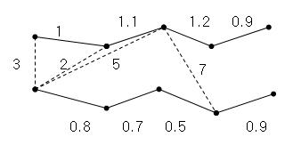 Fig 3-1

Can define clusters as the connected component of the similarity graph
=> Same result as "Single linkage algorithms"
$ X_i \sim X_j $ if there is chain
$ X_i \sim X_{i_1} \sim X_{i_2} \sim \cdots X_{i_k} \sim X_{j} $ complete
Can also define clusters as the maximal subgraphs of similarity graph
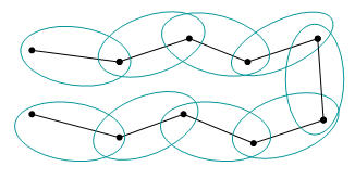 Fig 3-2

=>this yeilds more compact, less enlongated clusters
The approach above is not good for, say,
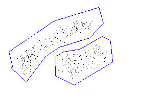 Fig 3-3