| (14 intermediate revisions by 3 users not shown) | |||
| Line 1: | Line 1: | ||
| − | [ | + | =Lecture 20, [[ECE662]]: Decision Theory= |
| + | |||
| + | Lecture notes for [[ECE662:BoutinSpring08_Old_Kiwi|ECE662 Spring 2008]], Prof. [[user:mboutin|Boutin]]. | ||
| + | |||
| + | Other lectures: [[Lecture 1 - Introduction_Old Kiwi|1]], | ||
| + | [[Lecture 2 - Decision Hypersurfaces_Old Kiwi|2]], | ||
| + | [[Lecture 3 - Bayes classification_Old Kiwi|3]], | ||
| + | [[Lecture 4 - Bayes Classification_Old Kiwi|4]], | ||
| + | [[Lecture 5 - Discriminant Functions_Old Kiwi|5]], | ||
| + | [[Lecture 6 - Discriminant Functions_Old Kiwi|6]], | ||
| + | [[Lecture 7 - MLE and BPE_Old Kiwi|7]], | ||
| + | [[Lecture 8 - MLE, BPE and Linear Discriminant Functions_Old Kiwi|8]], | ||
| + | [[Lecture 9 - Linear Discriminant Functions_Old Kiwi|9]], | ||
| + | [[Lecture 10 - Batch Perceptron and Fisher Linear Discriminant_Old Kiwi|10]], | ||
| + | [[Lecture 11 - Fischer's Linear Discriminant again_Old Kiwi|11]], | ||
| + | [[Lecture 12 - Support Vector Machine and Quadratic Optimization Problem_Old Kiwi|12]], | ||
| + | [[Lecture 13 - Kernel function for SVMs and ANNs introduction_Old Kiwi|13]], | ||
| + | [[Lecture 14 - ANNs, Non-parametric Density Estimation (Parzen Window)_Old Kiwi|14]], | ||
| + | [[Lecture 15 - Parzen Window Method_Old Kiwi|15]], | ||
| + | [[Lecture 16 - Parzen Window Method and K-nearest Neighbor Density Estimate_Old Kiwi|16]], | ||
| + | [[Lecture 17 - Nearest Neighbors Clarification Rule and Metrics_Old Kiwi|17]], | ||
| + | [[Lecture 18 - Nearest Neighbors Clarification Rule and Metrics(Continued)_Old Kiwi|18]], | ||
| + | [[Lecture 19 - Nearest Neighbor Error Rates_Old Kiwi|19]], | ||
| + | [[Lecture 20 - Density Estimation using Series Expansion and Decision Trees_Old Kiwi|20]], | ||
| + | [[Lecture 21 - Decision Trees(Continued)_Old Kiwi|21]], | ||
| + | [[Lecture 22 - Decision Trees and Clustering_Old Kiwi|22]], | ||
| + | [[Lecture 23 - Spanning Trees_Old Kiwi|23]], | ||
| + | [[Lecture 24 - Clustering and Hierarchical Clustering_Old Kiwi|24]], | ||
| + | [[Lecture 25 - Clustering Algorithms_Old Kiwi|25]], | ||
| + | [[Lecture 26 - Statistical Clustering Methods_Old Kiwi|26]], | ||
| + | [[Lecture 27 - Clustering by finding valleys of densities_Old Kiwi|27]], | ||
| + | [[Lecture 28 - Final lecture_Old Kiwi|28]], | ||
| + | ---- | ||
| + | ---- | ||
==Density Estimation using Series Expansion== | ==Density Estimation using Series Expansion== | ||
| Line 24: | Line 57: | ||
<math>p(x) \approx \sum _{j=0} ^{m} \frac{p^{(j)}(x)(x-x_0)^j}{j!}</math> (6) when <math>p(x) \in C^{m+1}(\Re)</math> | <math>p(x) \approx \sum _{j=0} ^{m} \frac{p^{(j)}(x)(x-x_0)^j}{j!}</math> (6) when <math>p(x) \in C^{m+1}(\Re)</math> | ||
| + | |||
| + | <math>p(x) \in C^{0}(\Re)</math> means continuous | ||
| + | <math>p(x) \in C^{1}(\Re)</math> means differentiable once and continuous order derivative | ||
| + | <math>p(x) \in C^{2}(\Re)</math> means differentiable twice and continuous second order derivative | ||
| + | |||
When m=1,linear approximation. | When m=1,linear approximation. | ||
<math>p(\vec{x})\approx c_0 + c \cdot (x-x_0)</math> (7) | <math>p(\vec{x})\approx c_0 + c \cdot (x-x_0)</math> (7) | ||
| + | |||
| + | |||
| + | [[Image:lec20_pic1_Old Kiwi.PNG]] | ||
| + | Figure 1 | ||
| + | |||
| + | |||
| + | * Take hair length samples for men | ||
| + | |||
| + | [[Image:lec20_pic2_Old Kiwi.PNG]] | ||
| + | Figure 2 | ||
| + | |||
| + | |||
Must use "Parzen window" approach to approximate <math>p(x)</math> | Must use "Parzen window" approach to approximate <math>p(x)</math> | ||
| Line 35: | Line 85: | ||
d is number of total samples | d is number of total samples | ||
| − | + | <math>V_d</math> is volume of that neighborhood | |
There is relationship between series expansion and Parzen Windows. | There is relationship between series expansion and Parzen Windows. | ||
| Line 79: | Line 129: | ||
<math>c_2 = - \frac{1}{h_d ^3}</math> (23) | <math>c_2 = - \frac{1}{h_d ^3}</math> (23) | ||
| − | |error| less than | + | |error| less than <math>\frac{1}{\sqrt{\pi}} \sum _{i=1} ^{d} \frac{{(x-x_i)}^4}{{h_d}^4 4!}= \frac{1}{\sqrt{\pi} 4!} \sum _{i=1} ^{d} \frac{{(x-x_i)}^4}{{h_d}^4}</math> |
| + | * This is samll when <math>\ | \frac{(x-x_i)}{h_d}|</math> is small for all i's | ||
| + | ==> Need to be within distance <math>\ h_d </math> of all of your samples | ||
| + | |||
| + | [[Image:lec20_pic3_Old Kiwi.PNG]] | ||
| + | Figure 3 | ||
==Decision Trees== | ==Decision Trees== | ||
| Line 97: | Line 152: | ||
[[Image:ECE662_lect20_tree1_Old Kiwi.jpg]] | [[Image:ECE662_lect20_tree1_Old Kiwi.jpg]] | ||
| − | |||
| + | [[Image:Lec20_mw_decbound_Old Kiwi.PNG]] | ||
| + | Figure 4 | ||
| + | |||
| + | [[Image:ECE662_lect20_tree2_Old Kiwi.jpg]] | ||
| − | + | [[Category:Lecture Notes]] | |
| − | [ | + | |
| − | + | ||
| − | + | ||
| − | + | ||
Latest revision as of 08:42, 17 January 2013
Lecture 20, ECE662: Decision Theory
Lecture notes for ECE662 Spring 2008, Prof. Boutin.
Other lectures: 1, 2, 3, 4, 5, 6, 7, 8, 9, 10, 11, 12, 13, 14, 15, 16, 17, 18, 19, 20, 21, 22, 23, 24, 25, 26, 27, 28,
Density Estimation using Series Expansion
Last "non-parametric" technique (although very parametric)
Write $ p(\vec{x})=\sum _{j=0}^{\infty}c_j f_j (\vec{x}) \cong \sum _{j=0} ^{m}c_j f_j (\vec{x}) $ (1)
where {$ fj's $} are pre-determined class of functions
$ \vec{x} = (x_1, \cdots, x_n) $ (2)
Monomials: $ x_1 , x_1x_2 , x_1 ^3 $ (3)
Polynomials: $ x_1 + x_2 , x_1 + x_1 ^2 +x_1 x_2 $ (4)
E.g.) Taylor expansion about $ x_0 $
In 1-D, $ p(x)=\sum _{j=1} ^ {\infty} \frac{p^{(j)} (x_0) (x-x_0)^j}{j!} $ (5) when $ p(x) $ is analytic
Taylor polynomial approximation
$ p(x) \approx \sum _{j=0} ^{m} \frac{p^{(j)}(x)(x-x_0)^j}{j!} $ (6) when $ p(x) \in C^{m+1}(\Re) $
$ p(x) \in C^{0}(\Re) $ means continuous
$ p(x) \in C^{1}(\Re) $ means differentiable once and continuous order derivative
$ p(x) \in C^{2}(\Re) $ means differentiable twice and continuous second order derivative
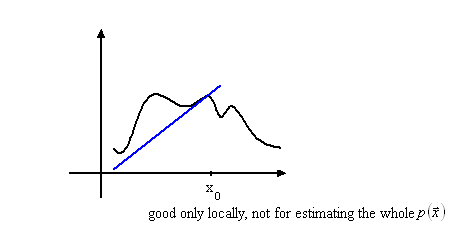
When m=1,linear approximation.
$ p(\vec{x})\approx c_0 + c \cdot (x-x_0) $ (7)
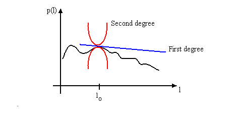
- Take hair length samples for men
Must use "Parzen window" approach to approximate $ p(x) $
$ p(x) \cong \frac{K}{dV_d} $ (8), where K is number of samples in a neighborhood of x
d is number of total samples
$ V_d $ is volume of that neighborhood
There is relationship between series expansion and Parzen Windows.
Recall window function $ \Phi (\vec{x}) $
<<Picuture>>
$ \Phi (\frac{\vec{x}-\vec{x}_i}{h_d}) $ (9) used in approximating $ p(x) $
$ p(\vec{x}) \cong p_d(\vec{x})=\sum _{i=1} ^{d} \frac{1}{dV_d} \Phi (\frac{\vec{x}-\vec{x}_i}{h_d}) $ (10)
Want $ p_d (\vec{x})\cong \sum _{j=1} ^{m} c_j (x_i , \cdots, x_d)f_j (\vec{x}) $ (11)
Write $ \Phi (\vec{x})= \sum _{j=1} ^{m} c_j (x_i , \cdots, x_d)f_j (\vec{x}) $ (12)
By computing the series for $ \Phi (\vec {x}) \cong \sum _{j=1} ^{m} \vec {c}_j f_j (\vec{x}) $ (13)
Example) 1D Gaussian window and Tayor expansion
$ \Phi (u) = \frac{1}{\sqrt{\pi}} e ^{-u^2} $ (14)
We have $ \Phi (u)= \frac{1}{\sqrt{\pi}} \sum _{j=0} ^{\infty} \frac{{(-1)}^j u^{2j}}{j!} $ with |error|$ \leq \frac{1}{\sqrt{\pi}} \frac{u^{2m+1}}{(m+1)!} $ (15)
So for m=1,
$ \Phi (\frac{x-x_i}{h_d}) \cong \frac{1}{\sqrt{\pi}} - \frac{1}{\sqrt{\pi}} (\frac{x-x_i}{h_d})^2 = \frac{1}{\sqrt{\pi}} + \frac{2}{h_d ^2 \sqrt{\pi}} x x_i - \frac{1}{\sqrt{\pi} h_d ^2} x^2 - \frac{1}{\sqrt{\pi} h_d ^2} x_i ^2 $ (16)
<<Picture>>
$ \tilde{c} _0 (x_i) = \frac{1}{\sqrt{\pi}} - \frac{1}{\sqrt{\pi} h_d ^2}x_i ^2 $ (17)
$ \tilde{c} _1 = \frac{2}{\sqrt{\pi} h_d ^2}x_i $ (18)
$ \tilde{c} _2 = - \frac{1}{\sqrt{\pi} h_d ^2} $ (19)
So $ p_d (\vec{x}) \cong \sum _{j=0} ^{2} (\frac{1}{dV_d}\sum _{i=1} ^{d}\tilde{c}_j (x_i)) x^j $ (20)
, where $ c_0 = \frac{1}{dV_d} \sum _{i=1} ^{d} \tilde {c}_0 (x_i) = \frac{1}{d h_d} (\sum _{i=1} ^{d} \frac{1}{\sqrt{\pi}}- \frac{1}{\sqrt{\pi}h_d ^2}x_i ^2) $ (21)
$ c_1 = \frac{1}{d V_d} \sum _{i=1} ^{d} \frac{2}{h_d ^2 \sqrt{\pi}}x_i $ (22)
$ c_2 = - \frac{1}{h_d ^3} $ (23)
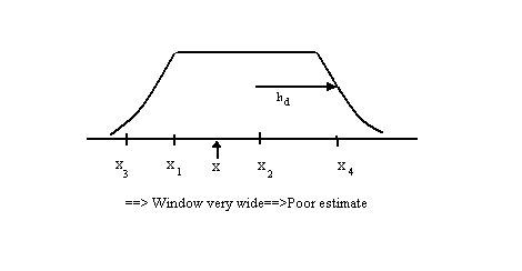
|error| less than $ \frac{1}{\sqrt{\pi}} \sum _{i=1} ^{d} \frac{{(x-x_i)}^4}{{h_d}^4 4!}= \frac{1}{\sqrt{\pi} 4!} \sum _{i=1} ^{d} \frac{{(x-x_i)}^4}{{h_d}^4} $
- This is samll when $ \ | \frac{(x-x_i)}{h_d}| $ is small for all i's
==> Need to be within distance $ \ h_d $ of all of your samples
Decision Trees
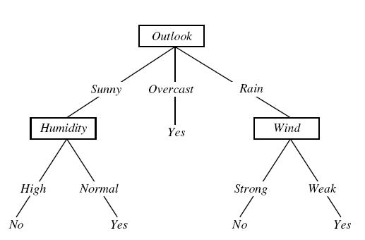
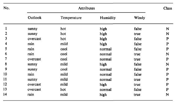
Reference DHS Chapter 8 Decision tree is one of the most powerful method for classification, because it simplifies the classification by dividing the problem into subproblems. A sample decision tree and training set from J.R. Quinlan (Induction of Decision Trees) can be given as follows:
The decision tree separates two classes. First class is "play tennis" and the second one is "do not play tennis". The decision tree tries to find the answer by asking several question. The purpose is to generate decision tree using the training data.
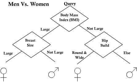
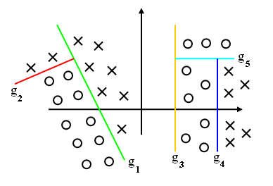
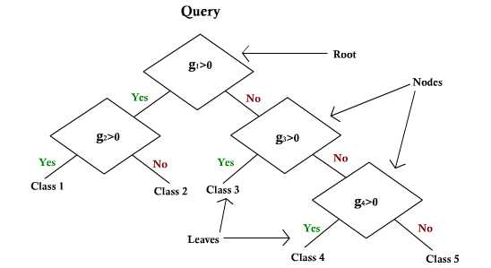
Instead of asking a complicated question $ g(x) >= 0 or <0 $
The idea: Ask a series of simple questions following a tree structure (linear 1-D).

