| (9 intermediate revisions by 2 users not shown) | |||
| Line 1: | Line 1: | ||
| + | =Lecture 17, [[ECE662]]: Decision Theory= | ||
| + | Lecture notes for [[ECE662:BoutinSpring08_Old_Kiwi|ECE662 Spring 2008]], Prof. [[user:mboutin|Boutin]]. | ||
| + | |||
| + | Other lectures: [[Lecture 1 - Introduction_Old Kiwi|1]], | ||
| + | [[Lecture 2 - Decision Hypersurfaces_Old Kiwi|2]], | ||
| + | [[Lecture 3 - Bayes classification_Old Kiwi|3]], | ||
| + | [[Lecture 4 - Bayes Classification_Old Kiwi|4]], | ||
| + | [[Lecture 5 - Discriminant Functions_Old Kiwi|5]], | ||
| + | [[Lecture 6 - Discriminant Functions_Old Kiwi|6]], | ||
| + | [[Lecture 7 - MLE and BPE_Old Kiwi|7]], | ||
| + | [[Lecture 8 - MLE, BPE and Linear Discriminant Functions_Old Kiwi|8]], | ||
| + | [[Lecture 9 - Linear Discriminant Functions_Old Kiwi|9]], | ||
| + | [[Lecture 10 - Batch Perceptron and Fisher Linear Discriminant_Old Kiwi|10]], | ||
| + | [[Lecture 11 - Fischer's Linear Discriminant again_Old Kiwi|11]], | ||
| + | [[Lecture 12 - Support Vector Machine and Quadratic Optimization Problem_Old Kiwi|12]], | ||
| + | [[Lecture 13 - Kernel function for SVMs and ANNs introduction_Old Kiwi|13]], | ||
| + | [[Lecture 14 - ANNs, Non-parametric Density Estimation (Parzen Window)_Old Kiwi|14]], | ||
| + | [[Lecture 15 - Parzen Window Method_Old Kiwi|15]], | ||
| + | [[Lecture 16 - Parzen Window Method and K-nearest Neighbor Density Estimate_Old Kiwi|16]], | ||
| + | [[Lecture 17 - Nearest Neighbors Clarification Rule and Metrics_Old Kiwi|17]], | ||
| + | [[Lecture 18 - Nearest Neighbors Clarification Rule and Metrics(Continued)_Old Kiwi|18]], | ||
| + | [[Lecture 19 - Nearest Neighbor Error Rates_Old Kiwi|19]], | ||
| + | [[Lecture 20 - Density Estimation using Series Expansion and Decision Trees_Old Kiwi|20]], | ||
| + | [[Lecture 21 - Decision Trees(Continued)_Old Kiwi|21]], | ||
| + | [[Lecture 22 - Decision Trees and Clustering_Old Kiwi|22]], | ||
| + | [[Lecture 23 - Spanning Trees_Old Kiwi|23]], | ||
| + | [[Lecture 24 - Clustering and Hierarchical Clustering_Old Kiwi|24]], | ||
| + | [[Lecture 25 - Clustering Algorithms_Old Kiwi|25]], | ||
| + | [[Lecture 26 - Statistical Clustering Methods_Old Kiwi|26]], | ||
| + | [[Lecture 27 - Clustering by finding valleys of densities_Old Kiwi|27]], | ||
| + | [[Lecture 28 - Final lecture_Old Kiwi|28]], | ||
| + | ---- | ||
| + | ---- | ||
'''Nearest Neighbor Classification Rule''' | '''Nearest Neighbor Classification Rule''' | ||
* useful when there are several labels | * useful when there are several labels | ||
| Line 24: | Line 57: | ||
[[Image:distances_Old Kiwi.jpg]] | [[Image:distances_Old Kiwi.jpg]] | ||
| − | ''' | + | '''Illustration of 3 different metrics''' |
| Line 31: | Line 64: | ||
Euclidean distance: <math>D(\vec{x_1},\vec{x_2})=||\vec{x_1}-\vec{x_2}||_{L_2}=\sqrt{\sum_{i=1}^n ({x_1}^i-{x_2}^i)^2}</math> | Euclidean distance: <math>D(\vec{x_1},\vec{x_2})=||\vec{x_1}-\vec{x_2}||_{L_2}=\sqrt{\sum_{i=1}^n ({x_1}^i-{x_2}^i)^2}</math> | ||
| − | Manhattan distance: <math>D(\vec{x_1},\vec{x_2})=||\vec{x_1}-\vec{x_2}||_{L_1}=\sum_{i=1}^n |{x_1}^i-{x_2}^i|</math> | + | Manhattan (cab driver) distance: <math>D(\vec{x_1},\vec{x_2})=||\vec{x_1}-\vec{x_2}||_{L_1}=\sum_{i=1}^n |{x_1}^i-{x_2}^i|</math> |
Minkowski metric: <math>D(\vec{x_1},\vec{x_2})=||\vec{x_1}-\vec{x_2}||_{L_p}=(\sum_{i=1}^n ({x_1}^i-{x_2}^i)^p)^{\frac{1}{p}}</math> | Minkowski metric: <math>D(\vec{x_1},\vec{x_2})=||\vec{x_1}-\vec{x_2}||_{L_p}=(\sum_{i=1}^n ({x_1}^i-{x_2}^i)^p)^{\frac{1}{p}}</math> | ||
Riemannian metric: <math>D(\vec{x_1},\vec{x_2})=\sqrt{(\vec{x_1}-\vec{x_2})^\top \mathbb{M}(\vec{x_1}-\vec{x_2})}</math> | Riemannian metric: <math>D(\vec{x_1},\vec{x_2})=\sqrt{(\vec{x_1}-\vec{x_2})^\top \mathbb{M}(\vec{x_1}-\vec{x_2})}</math> | ||
| + | |||
| + | Infinite norm: <math>D(\vec{x_1},\vec{x_2})=||\vec{x_1}-\vec{x_2}||_{\infty}=max_i |{x_1}^i-{x_2}^i|</math> | ||
| + | |||
where M is a symmetric positive definite <math>n\times n</math> matrix. Different choices for M enable associating different weights with different components. | where M is a symmetric positive definite <math>n\times n</math> matrix. Different choices for M enable associating different weights with different components. | ||
| Line 67: | Line 103: | ||
becasue shape defined by point is unchanged (invariant) by rotation and translation of triangles. | becasue shape defined by point is unchanged (invariant) by rotation and translation of triangles. | ||
| − | Therefore, distance between 2 triangles (or shapes) must be | + | Therefore, distance between 2 triangles (or shapes) must be independent on the position and orientation of triangles. |
'''Procrustes metric''' | '''Procrustes metric''' | ||
| Line 92: | Line 128: | ||
(p1,p2,p3) -> (new p1, new p2, new p3) | (p1,p2,p3) -> (new p1, new p2, new p3) | ||
| − | + | ---- | |
| + | [[ECE662:BoutinSpring08_Old_Kiwi|Back to ECE662, Spring 2008, Prof. Boutin]] | ||
[[Category:Lecture Notes]] | [[Category:Lecture Notes]] | ||
Latest revision as of 08:38, 17 January 2013
Lecture 17, ECE662: Decision Theory
Lecture notes for ECE662 Spring 2008, Prof. Boutin.
Other lectures: 1, 2, 3, 4, 5, 6, 7, 8, 9, 10, 11, 12, 13, 14, 15, 16, 17, 18, 19, 20, 21, 22, 23, 24, 25, 26, 27, 28,
Nearest Neighbor Classification Rule
- useful when there are several labels
- e.g. fingerprint-based recognition
Problem: Given the labeled training samples: $ \vec{X_1}, \vec{X_2}, \ldots, \vec{X_d} $ $ \in \mathbb{R}^n $ (or some other feature space) and an unlabeled test point $ \vec{X_0} $ $ \in \mathbb{R}^n $.
Classification: Let $ \vec{X_i} $ be the closest training point to $ \vec{X_0} $, then we assign the class of $ \vec{X_i} $ to $ \vec{X_0} $.
What do we mean by closest?
There are many meaning depending on the metric we choose for the feature space.
Definition A "metric" on a space S is a function
$ D: S\times S\rightarrow \mathbb{R} $
that satisfies the following 4 properties:
- Non-negativity $ D(\vec{x_1},\vec{x_2})\geq 0, \forall \vec{x_1},\vec{x_2}\in S $
- Symmetry $ D(\vec{x_1},\vec{x_2})=D(\vec{x_2},\vec{x_1}), \forall \vec{x_1},\vec{x_2}\in S $
- Reflexivity $ D(\vec{x},\vec{x})=0, \forall \vec{x}\in S $
- Triangle Inequality $ D(\vec{x_1},\vec{x_2})+D(\vec{x_2},\vec{x_3})\geq D(\vec{x_1},\vec{x_3}) , \forall \vec{x_1}, \vec{x_2}, \vec{x_3}\in S $
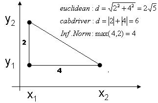
 Illustration of 3 different metrics
Examples of metrics
Euclidean distance: $ D(\vec{x_1},\vec{x_2})=||\vec{x_1}-\vec{x_2}||_{L_2}=\sqrt{\sum_{i=1}^n ({x_1}^i-{x_2}^i)^2} $
Manhattan (cab driver) distance: $ D(\vec{x_1},\vec{x_2})=||\vec{x_1}-\vec{x_2}||_{L_1}=\sum_{i=1}^n |{x_1}^i-{x_2}^i| $
Minkowski metric: $ D(\vec{x_1},\vec{x_2})=||\vec{x_1}-\vec{x_2}||_{L_p}=(\sum_{i=1}^n ({x_1}^i-{x_2}^i)^p)^{\frac{1}{p}} $
Riemannian metric: $ D(\vec{x_1},\vec{x_2})=\sqrt{(\vec{x_1}-\vec{x_2})^\top \mathbb{M}(\vec{x_1}-\vec{x_2})} $
Infinite norm: $ D(\vec{x_1},\vec{x_2})=||\vec{x_1}-\vec{x_2}||_{\infty}=max_i |{x_1}^i-{x_2}^i| $
where M is a symmetric positive definite $ n\times n $ matrix. Different choices for M enable associating different weights with different components.
In this way, we see that $ \mathbb{R}^n $, $ \mathbb{Z}^n $, $ \mathbb{C}^n $ have many natural metrics, but feature could be in some other set, e.g. a discrete set.
for example,
$ x_1 $={fever, skinrash, high blodd pressure}
$ x_2 $={fever, neckstiffness}
Tanimoto metric
$ D(set1, set2) = \frac {|set1|+|set2|-2|set1 \bigcap set2| }{|set1|+|set2|-|set1 \bigcap set2|} $
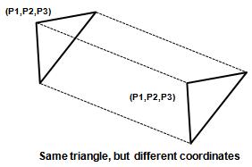
Example: previous approach to shape recognition Given is a set of ordered points in $ R_n =(p_1,p_2,\cdots,p_N) $ We want to recognize the shape
Given template (triangle form): (T1,T2,...,TN); We want to assign one of test template to a test (P1,P2,P3) In this case, we should not use Euclidean distance!,
becasue shape defined by point is unchanged (invariant) by rotation and translation of triangles.
Therefore, distance between 2 triangles (or shapes) must be independent on the position and orientation of triangles.
Procrustes metric
$ D(p,\bar p)= \sum_{\begin{matrix}i=1 \\ rotation R, translation T \end{matrix}}^n {\begin{Vmatrix} Rp_i+T-\bar p_i \end{Vmatrix}} _{L^2} $
$ p=(p_1, p_2, \cdots ,p_N),\bar p = (\bar p_1, \bar p_2, \cdots ,\bar p_N) $
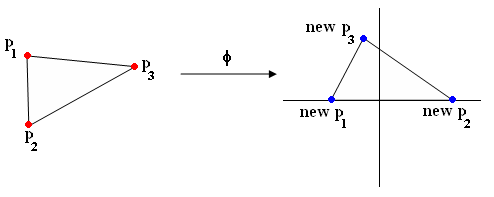
Alternative approach "Use invariant coordinate to repeat $ p=(p_1, p_2, \cdots ,p_N) $ "
i.e find $ \varphi $ such that
$ \varphi : \mathbb{R}^n\rightarrow \mathbb{R}^k $ (where, typically $ k \leq n $)
s.t $ \varphi (x) = \varphi (\bar x) $
whenever $ \exists $ R, T with $ R \bar X + \bar T = X $
Example of phi with triangle (Figure 3):

(p1,p2,p3) -> (new p1, new p2, new p3)


