Estimation Using Nearest Neighbor - Rhea

Introduction

In this slecture, basic principles of implementing nearest neighbor rule will be covered. The error related to the nearest neighbor rule will be discussed in detail including convergence, error rate, and error bound. Since the nearest neighbor rule relies on metric function between patterns, the properties of metrics will be studied in detail. Example of different metrics will be introduced with its characteristics. The representative of real application such as body posture recognition using Procrustes metric could be a good example to understand the nearest neighbor rule.----

Nearest Neighbor Basic Principle

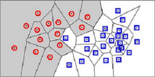
Let's consider a testing sample x. Based on labeled training sample $ D^n = x_{1},... ,x_{n}, $ the nearest neighbor technique will find the closest point x' to x. Then we assign the class of x' to x. This is how the classification based on the nearest neighbor rule is processed. Although this rule is very simple, it is also reasonable. The label $ \theta' $ used in the nearest neighbor is random variable which means $\theta' = w_{i}$ is same as a posteriori probability $P(w_{i}|x').$ If sample sizes are big enough, it could be assumed that x' is sufficiently close to x that $ P(w_{i}|x') = P(w_{i}|x). $ Using the nearest neighbor rule, we could get high accuracy classification if sample sizes are guaranteed. In other words, the nearest neighbor rule is matching perfectly with probabilities in nature.

Error Rate & Bound using NN

In order to find the error rate and bound related to the nearest neighbor rule, we need to confirm the convergence of the nearest neighbor as sample increases to the infinity. We set $ P = \lim_{n \to \infty}P_n(e) $. Then, we set infinite sample conditional average probability of error as $ P(e|x) $. Using this the unconditional average probability of error which indicates the average error according to training samples can be shown as

Since minimum error caused by the nearest neighbor cannot be lower than error from Bayes decision rule, the minimum possible value of the error $P^*(e|x)$ can be represented as

Metrics Type

However, the closest distance between x' and x is determined by which metrics are used for feature space. A "metric" on a space S is a function $ D: S\times S\rightarrow \mathbb{R} $ which has following 4 properties:

• Non-negativity : $ D(\vec{x_{1}},\vec{x_{2}}) \geq 0, \forall \vec{x_{1}},\vec{x_{2}} \in S $
• Symmetry : $ D(\vec{x_{1}},\vec{x_{2}}) = D(\vec{x_{2}},\vec{x_{1}}), \forall \vec{x_{1}},\vec{x_{2}} \in S $
• Reflexivity : $ D(\vec{x},\vec{x}) = 0, \forall \vec{x} \in S $
• Triangle Inequality : $ D(\vec{x_{1}},\vec{x_{2}}) + D(\vec{x_{2}},\vec{x_{3}}) \geq D(\vec{x_{1}},\vec{x_{3}}), \forall \vec{x_{1}},\vec{x_{2}},\vec{x_{3}} \in S $

Real Application

References

Questions and comments

If you have any questions, comments, etc. please post them on this page.

Back to ECE662, Spring 2014