| (2 intermediate revisions by the same user not shown) | |||
| Line 1: | Line 1: | ||
[[Category:ECE438 (BoutinFall2009)]] | [[Category:ECE438 (BoutinFall2009)]] | ||
| + | [[Category:discrete-space Fourier transform]] | ||
| − | = | + | =DSFT of some basic filters= |
| − | + | Used in [[ECE438]] | |
| + | ---- | ||
Plot of the frequency response of the average filter: | Plot of the frequency response of the average filter: | ||
| Line 24: | Line 26: | ||
\right] | \right] | ||
</math> | </math> | ||
| − | + | ||
[[Image:edgedetectfilterfrequencyresponse.png]] | [[Image:edgedetectfilterfrequencyresponse.png]] | ||
| − | Plot of the frequency response of the filter: | + | Plot of the frequency response of the following filter, with <math>\lambda = 0.5</math>.: |
<math> | <math> | ||
| Line 45: | Line 47: | ||
---- | ---- | ||
| − | [[ ECE438 (BoutinFall2009)|Back to ECE438 | + | [[2010_Fall_ECE_438_Boutin|Back to ECE438 Fall 2010]] |
| + | |||
| + | [[ ECE438 (BoutinFall2009)|Back to ECE438 Fall2009]] | ||
Latest revision as of 12:50, 26 November 2014
DSFT of some basic filters
Used in ECE438
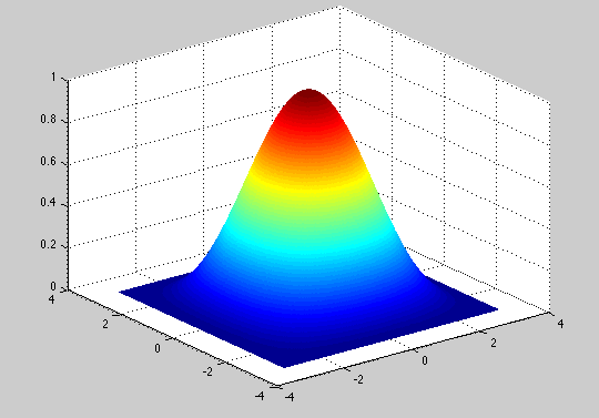
Plot of the frequency response of the average filter:
$ h(k,l)=\frac{1}{16}\left[ \begin{array}{ccc}1& 2 & 1\\ 2 &4 &2 \\ 1 & 2 & 1 \end{array} \right] $
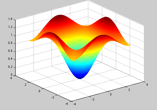
Plot of the frequency response of the filter:
$ h(k,l)=\frac{1}{9}\left[\begin{array}{ccc}-1& -1 & -1\\ -1 &8 &-1 \\ -1 & -1 & -1 \end{array} \right] $
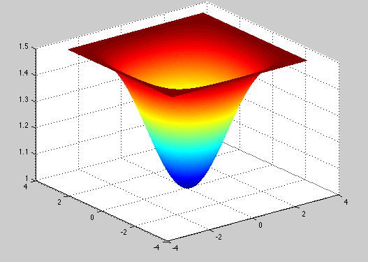
Plot of the frequency response of the following filter, with $ \lambda = 0.5 $.:
$ h(k,l)=\frac{1}{9}\left[\begin{array}{ccc}-\lambda & -\lambda & -\lambda\\ -\lambda &9+8 \lambda & -\lambda \\ -\lambda & -\lambda & -\lambda \end{array} \right] $
Links
- Example of unsharp masking applied to eye image
- Illustrations of grainy effects caused by unsharp mark


