| (One intermediate revision by one other user not shown) | |||
| Line 1: | Line 1: | ||
| − | |||
| − | = | + | = Illustrations of the Central Limit Theorem = |
| + | Put your content here . . . | ||
| + | The CLT assume that given a population of i.i.d N random values with mean <span class="texhtml">μ</span> and finite standard deviation <span class="texhtml">σ</span>, and suppose that we draw random samples of size n from that population, such as we draw many samples from the population each sample has a mean, then the CLT says that the distribution of the sample means is normal regardless of the population distribution. | ||
| − | + | To illustrate the beauty of the CLT i wrote a mat-lab code that generate a population of (512000) i.i.d random values which can be sampled from one of the following five distribution: | |
| + | 1.Exponential distribution with mean <span class="texhtml">μ</span> | ||
| + | 2.Uniform distribution in the range [a,b] where a<b | ||
| + | 3.Chi-squared distribution with v degrees of freedom | ||
| − | [[ 2010 Spring ECE 662 mboutin|Back to 2010 Spring ECE 662 mboutin]] | + | 4.Normal distribution with mean <span class="texhtml">μ</span> and standard deviation <span class="texhtml">σ</span> |
| + | |||
| + | 5.Log Normal distribution with mean <span class="texhtml">μ</span> and standard deviation <span class="texhtml">σ</span> | ||
| + | |||
| + | <br> Then 1000 samples were drawn in an increasing sizes such as: | ||
| + | |||
| + | the first 1000 samples each sample has size n = 1 | ||
| + | |||
| + | the second 1000 samples each sample has size n = 2 | ||
| + | |||
| + | . | ||
| + | |||
| + | . | ||
| + | |||
| + | . | ||
| + | |||
| + | the nine'th 1000 samples each sample has size n = 512 | ||
| + | |||
| + | and finally a histogram and normal plot were constructed for each sample size. | ||
| + | |||
| + | <br> For example consider that our population was generated from an exponential distribution with mean <span class="texhtml">μ = 5</span> then our set of all samples will look like: | ||
| + | |||
| + | <br> | ||
| + | |||
| + | [[Image:Untitled.JPG|830x340px]]<br> | ||
| + | |||
| + | '''notice '''here each row represents a sample of size n=512 "# columns " and we have 1000 samples "# rows". | ||
| + | |||
| + | The histogram and Normal plots are given below: | ||
| + | |||
| + | [[Image:HistExpo.jpg|1200x800px]]<br> | ||
| + | |||
| + | so from the histogram above we can see that as the size of the sample increase the distribution of the '''sample means approach approximately to a normal distribution with mean <span class="texhtml">μ</span> =5 which is the same as the mean of the original population and a standard deviation <span class="texhtml">σ' = σ / ''s'''</span>'''''q''''r''''t''(''n''). | ||
| + | |||
| + | also we can see from the normal plots below that for small number n the plot will have a curvature because the original distribution was not Normal , but as n increase the plot approach to a linear shape as illustrated below. | ||
| + | |||
| + | [[Image:NorPlotExp.jpg|1200x900px]] | ||
| + | |||
| + | <br> | ||
| + | |||
| + | more clarifications about this topic will be in my HW#1 report , and below is the matlab source code for the above experiment: | ||
| + | |||
| + | function CLT(popDist,distParameters)<br>% <br>% Input:<br>% popDist: a number represent the distribution of the population<br>% 1 : exponentioal distribution <br>% 2 : uniform distribution <br>% 3 : chi-square distribution<br>% 4 : normal distribution<br>% 5 : log normal distribuion<br>% <br>% distParameters: this represents a vector that conatins the<br>% parameters of the distribution<br>% 1 : exponentioal distribution [mean]<br>% 2 : uniform distribution [min value; max value]<br>% 3 : Chi distribution [ v degrees of freedom]<br>% 4 : normal distribution [mean; standard deviation]<br>% 5 : log normal distribuion [mean; standard deviation]<br>% usage examples:<br>% example1: CLT(1,[5]);<br>% example2: CLT(2,[0;5]);<br>% example3: CLT(3,[5]);<br>% example4: CLT(4,[2;5])<br>% example5: CLT(5,[2;5]);<br>% <br>% written by Rami Alazrai 2/22/2010. | ||
| + | |||
| + | close all<br>nSamples=1000; | ||
| + | |||
| + | if(popDist == 1)%exponential<br>mu = distParameters(1);<br>nMax = 512;<br>setOfSamples = exprnd(mu,nSamples,nMax);<br>figure<br>X = 0:0.01:15;<br>plot(X, exppdf(X,mu),'r.');<br>strMu = num2str(mu);<br>str = strcat('Exponential distribution of the population with mean = ',strMu);<br>title( str);<br>xlabel('x');<br>ylabel('Exponential pdf'); | ||
| + | |||
| + | elseif(popDist == 2)%uniform<br>a = distParameters(1);<br>b = distParameters(2);<br>nMax = 512;<br>setOfSamples = unifrnd(a,b,nSamples,nMax); <br>figure<br>X = 0:0.01:15;<br>plot(X, unifpdf(X,a,b),'r.');<br>stra = num2str(a);<br>strb = num2str(b);<br>str = strcat('Uniform distribution of the population with a = ',stra,' and b = ', strb);<br>title( str);<br>xlabel('x');<br>ylabel('Uniform pdf'); | ||
| + | |||
| + | elseif(popDist == 3)%chi-squared<br>v = distParameters(1);<br>nMax = 512;<br>setOfSamples = chi2rnd(v,nSamples,nMax); <br>figure<br>X = 0:0.01:15;<br>plot(X, chi2pdf(X,v),'r.');<br>strv = num2str(v);<br>str = strcat('Chi-squared distribution of the population with v = ',strv);<br>title( str);<br>xlabel('x');<br>ylabel('Chi-squared pdf'); | ||
| + | |||
| + | elseif(popDist == 4)%normal<br>mu = distParameters(1);<br>sigma = distParameters(2);<br>nMax = 512;<br>setOfSamples = normrnd(mu,sigma,nSamples,nMax);<br>figure<br>X = -4*sigma:0.01:4*sigma;<br>plot(X, normpdf(X,mu,sigma),'r.');<br>stra = num2str(mu);<br>strb = num2str(sigma);<br>str = strcat('Normal distribution of the population with mean = ',stra,' and standard deviation = ', strb);<br>title( str);<br>xlabel('x');<br>ylabel('Normal pdf'); | ||
| + | |||
| + | elseif(popDist == 5)%log normal<br>mu = distParameters(1);<br>sigma = distParameters(2);<br>nMax = 10000;<br>setOfSamples = normrnd(mu,sigma,nSamples,nMax);<br>figure<br>X = 0:0.001:4*sigma;<br>plot(X, normpdf(X,mu,sigma),'r.');<br>stra = num2str(mu);<br>strb = num2str(sigma);<br>str = strcat('LOG Normal distribution of the population with mean = ',stra,' and standard deviation = ', strb);<br>title( str);<br>xlabel('x');<br>ylabel('LOG Normal pdf'); | ||
| + | |||
| + | end <br>sampleMeans = zeros(nSamples,1,9);<br>for i = 0:8<br> sampleMeans(:,:,i+1) = sum(setOfSamples(:,1:(2^(i))),2)/(2^(i));<br>end<br>figure<br>subplot(2,4,1), hist(sampleMeans(:,:,1)),title('frequancy of sample means when n=1')<br>subplot(2,4,2), hist(sampleMeans(:,:,3)),title('frequancy of sample means when n=4')<br>subplot(2,4,3), hist(sampleMeans(:,:,4)),title('frequancy of sample means when n=16')<br>subplot(2,4,4), hist(sampleMeans(:,:,5)),title('frequancy of sample means when n=32')<br>subplot(2,4,5), hist(sampleMeans(:,:,6)),title('frequancy of sample means when n=64')<br>subplot(2,4,6), hist(sampleMeans(:,:,7)),title('frequancy of sample means when n=128')<br>subplot(2,4,7), hist(sampleMeans(:,:,8)),title('frequancy of sample means when n=256')<br>subplot(2,4,8), hist(sampleMeans(:,:,9)),title('frequancy of sample means when n=512')<br>figure<br>subplot(2,4,1), normplot(sampleMeans(:,:,1)),title('Normal Probability plot when the sample size n=1')<br>subplot(2,4,2), normplot(sampleMeans(:,:,3)),title('Normal Probability plot when the sample size n=4')<br>subplot(2,4,3), normplot(sampleMeans(:,:,4)),title('Normal Probability plot when the sample size n=16')<br>subplot(2,4,4), normplot(sampleMeans(:,:,5)),title('Normal Probability plot when the sample size n=32')<br>subplot(2,4,5), normplot(sampleMeans(:,:,6)),title('Normal Probability plot when the sample size n=64')<br>subplot(2,4,6), normplot(sampleMeans(:,:,7)),title('Normal Probability plot when the sample size n=128')<br>subplot(2,4,7), normplot(sampleMeans(:,:,8)),title('Normal Probability plot when the sample size n=256')<br>subplot(2,4,8), normplot(sampleMeans(:,:,9)),title('Normal Probability plot when the sample size n=512') | ||
| + | |||
| + | <br> <br> | ||
| + | --[[User:Ralazrai|Ralazrai]] 11:44, 23 February 2010 (UTC) | ||
| + | ---- | ||
| + | |||
| + | [[2010 Spring ECE 662 mboutin|Back to 2010 Spring ECE 662 mboutin]] | ||
| + | |||
| + | [[Category:2010_Spring_ECE_662_mboutin]] | ||
Latest revision as of 07:44, 23 February 2010
Illustrations of the Central Limit Theorem
Put your content here . . .
The CLT assume that given a population of i.i.d N random values with mean μ and finite standard deviation σ, and suppose that we draw random samples of size n from that population, such as we draw many samples from the population each sample has a mean, then the CLT says that the distribution of the sample means is normal regardless of the population distribution.
To illustrate the beauty of the CLT i wrote a mat-lab code that generate a population of (512000) i.i.d random values which can be sampled from one of the following five distribution:
1.Exponential distribution with mean μ
2.Uniform distribution in the range [a,b] where a<b
3.Chi-squared distribution with v degrees of freedom
4.Normal distribution with mean μ and standard deviation σ
5.Log Normal distribution with mean μ and standard deviation σ
Then 1000 samples were drawn in an increasing sizes such as:
the first 1000 samples each sample has size n = 1
the second 1000 samples each sample has size n = 2
.
.
.
the nine'th 1000 samples each sample has size n = 512
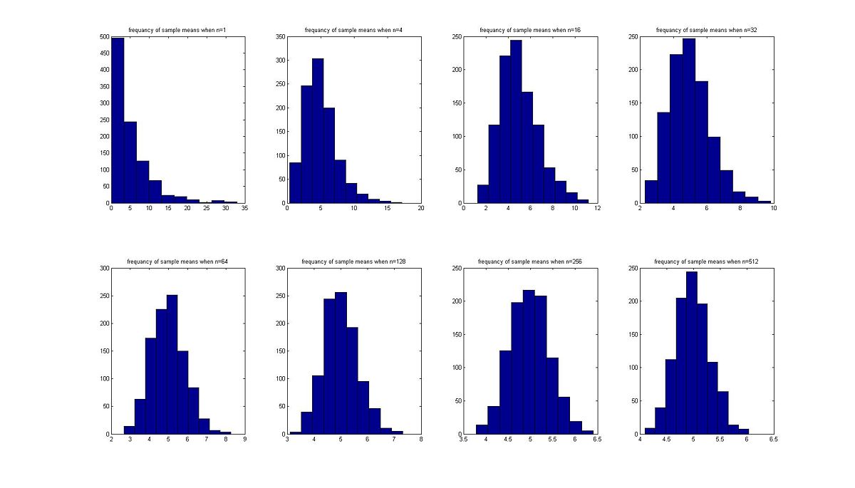
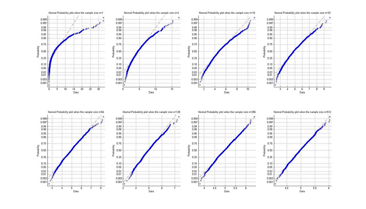
and finally a histogram and normal plot were constructed for each sample size.
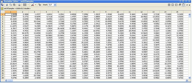
For example consider that our population was generated from an exponential distribution with mean μ = 5 then our set of all samples will look like:
notice here each row represents a sample of size n=512 "# columns " and we have 1000 samples "# rows".
The histogram and Normal plots are given below:
so from the histogram above we can see that as the size of the sample increase the distribution of the sample means approach approximately to a normal distribution with mean μ =5 which is the same as the mean of the original population and a standard deviation σ' = σ / s'q'r't(n).
also we can see from the normal plots below that for small number n the plot will have a curvature because the original distribution was not Normal , but as n increase the plot approach to a linear shape as illustrated below.
more clarifications about this topic will be in my HW#1 report , and below is the matlab source code for the above experiment:
function CLT(popDist,distParameters)
%
% Input:
% popDist: a number represent the distribution of the population
% 1 : exponentioal distribution
% 2 : uniform distribution
% 3 : chi-square distribution
% 4 : normal distribution
% 5 : log normal distribuion
%
% distParameters: this represents a vector that conatins the
% parameters of the distribution
% 1 : exponentioal distribution [mean]
% 2 : uniform distribution [min value; max value]
% 3 : Chi distribution [ v degrees of freedom]
% 4 : normal distribution [mean; standard deviation]
% 5 : log normal distribuion [mean; standard deviation]
% usage examples:
% example1: CLT(1,[5]);
% example2: CLT(2,[0;5]);
% example3: CLT(3,[5]);
% example4: CLT(4,[2;5])
% example5: CLT(5,[2;5]);
%
% written by Rami Alazrai 2/22/2010.
close all
nSamples=1000;
if(popDist == 1)%exponential
mu = distParameters(1);
nMax = 512;
setOfSamples = exprnd(mu,nSamples,nMax);
figure
X = 0:0.01:15;
plot(X, exppdf(X,mu),'r.');
strMu = num2str(mu);
str = strcat('Exponential distribution of the population with mean = ',strMu);
title( str);
xlabel('x');
ylabel('Exponential pdf');
elseif(popDist == 2)%uniform
a = distParameters(1);
b = distParameters(2);
nMax = 512;
setOfSamples = unifrnd(a,b,nSamples,nMax);
figure
X = 0:0.01:15;
plot(X, unifpdf(X,a,b),'r.');
stra = num2str(a);
strb = num2str(b);
str = strcat('Uniform distribution of the population with a = ',stra,' and b = ', strb);
title( str);
xlabel('x');
ylabel('Uniform pdf');
elseif(popDist == 3)%chi-squared
v = distParameters(1);
nMax = 512;
setOfSamples = chi2rnd(v,nSamples,nMax);
figure
X = 0:0.01:15;
plot(X, chi2pdf(X,v),'r.');
strv = num2str(v);
str = strcat('Chi-squared distribution of the population with v = ',strv);
title( str);
xlabel('x');
ylabel('Chi-squared pdf');
elseif(popDist == 4)%normal
mu = distParameters(1);
sigma = distParameters(2);
nMax = 512;
setOfSamples = normrnd(mu,sigma,nSamples,nMax);
figure
X = -4*sigma:0.01:4*sigma;
plot(X, normpdf(X,mu,sigma),'r.');
stra = num2str(mu);
strb = num2str(sigma);
str = strcat('Normal distribution of the population with mean = ',stra,' and standard deviation = ', strb);
title( str);
xlabel('x');
ylabel('Normal pdf');
elseif(popDist == 5)%log normal
mu = distParameters(1);
sigma = distParameters(2);
nMax = 10000;
setOfSamples = normrnd(mu,sigma,nSamples,nMax);
figure
X = 0:0.001:4*sigma;
plot(X, normpdf(X,mu,sigma),'r.');
stra = num2str(mu);
strb = num2str(sigma);
str = strcat('LOG Normal distribution of the population with mean = ',stra,' and standard deviation = ', strb);
title( str);
xlabel('x');
ylabel('LOG Normal pdf');
end
sampleMeans = zeros(nSamples,1,9);
for i = 0:8
sampleMeans(:,:,i+1) = sum(setOfSamples(:,1:(2^(i))),2)/(2^(i));
end
figure
subplot(2,4,1), hist(sampleMeans(:,:,1)),title('frequancy of sample means when n=1')
subplot(2,4,2), hist(sampleMeans(:,:,3)),title('frequancy of sample means when n=4')
subplot(2,4,3), hist(sampleMeans(:,:,4)),title('frequancy of sample means when n=16')
subplot(2,4,4), hist(sampleMeans(:,:,5)),title('frequancy of sample means when n=32')
subplot(2,4,5), hist(sampleMeans(:,:,6)),title('frequancy of sample means when n=64')
subplot(2,4,6), hist(sampleMeans(:,:,7)),title('frequancy of sample means when n=128')
subplot(2,4,7), hist(sampleMeans(:,:,8)),title('frequancy of sample means when n=256')
subplot(2,4,8), hist(sampleMeans(:,:,9)),title('frequancy of sample means when n=512')
figure
subplot(2,4,1), normplot(sampleMeans(:,:,1)),title('Normal Probability plot when the sample size n=1')
subplot(2,4,2), normplot(sampleMeans(:,:,3)),title('Normal Probability plot when the sample size n=4')
subplot(2,4,3), normplot(sampleMeans(:,:,4)),title('Normal Probability plot when the sample size n=16')
subplot(2,4,4), normplot(sampleMeans(:,:,5)),title('Normal Probability plot when the sample size n=32')
subplot(2,4,5), normplot(sampleMeans(:,:,6)),title('Normal Probability plot when the sample size n=64')
subplot(2,4,6), normplot(sampleMeans(:,:,7)),title('Normal Probability plot when the sample size n=128')
subplot(2,4,7), normplot(sampleMeans(:,:,8)),title('Normal Probability plot when the sample size n=256')
subplot(2,4,8), normplot(sampleMeans(:,:,9)),title('Normal Probability plot when the sample size n=512')
--Ralazrai 11:44, 23 February 2010 (UTC)


