| Line 11: | Line 11: | ||
---- | ---- | ||
| + | |||
We will now learn how to represent conditional probabilities using the cdf/pdf/pmf. This will provide us some of the most powerful tools for working with random variables: the conditional pdf and conditional pmf. | We will now learn how to represent conditional probabilities using the cdf/pdf/pmf. This will provide us some of the most powerful tools for working with random variables: the conditional pdf and conditional pmf. | ||
| Line 62: | Line 63: | ||
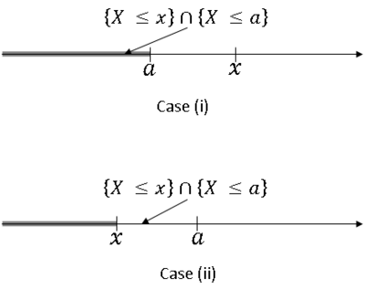
* Case (ii): <math>x>a</math><br/> | * Case (ii): <math>x>a</math><br/> | ||
<center><math>F_X(x|B) = \frac{P(X\leq x)}{P(X\leq a} = \frac{F_X(x)}{F_X(a)}</math></center> | <center><math>F_X(x|B) = \frac{P(X\leq x)}{P(X\leq a} = \frac{F_X(x)}{F_X(a)}</math></center> | ||
| + | |||
<center>[[Image:fig1_rv__conditional_distributions.png|400px|thumb|left|Fig 1: ''{X ≤ x} ∩ {X ≤ a}'' for the two different cases.]]</center> | <center>[[Image:fig1_rv__conditional_distributions.png|400px|thumb|left|Fig 1: ''{X ≤ x} ∩ {X ≤ a}'' for the two different cases.]]</center> | ||
| Line 74: | Line 76: | ||
<center>[[Image:fig2_rv__conditional_distributions.png|400px|thumb|left|Fig 2: f<math>_X</math>(x) and f<math>_X</math>(x<math>|</math>X ≤ a).]]</center> | <center>[[Image:fig2_rv__conditional_distributions.png|400px|thumb|left|Fig 2: f<math>_X</math>(x) and f<math>_X</math>(x<math>|</math>X ≤ a).]]</center> | ||
| + | |||
Bayes' Theorem for continuous X:<br/> | Bayes' Theorem for continuous X:<br/> | ||
| Line 83: | Line 86: | ||
but what we often want to know is a probability of the type P(''A''|''X''=''x'') for some ''A''∈''F''. We could define this as <br/> | but what we often want to know is a probability of the type P(''A''|''X''=''x'') for some ''A''∈''F''. We could define this as <br/> | ||
<center><math>P(A|X=x)\equiv\frac{P(A\cap \{X=x\})}{P(X=x)}</math></center> | <center><math>P(A|X=x)\equiv\frac{P(A\cap \{X=x\})}{P(X=x)}</math></center> | ||
| − | |||
but the right hand side (rhs) would be 0/0 since ''X'' is continuous. <br/> | but the right hand side (rhs) would be 0/0 since ''X'' is continuous. <br/> | ||
Instead, we will use the following definition in this case:<br/> | Instead, we will use the following definition in this case:<br/> | ||
| Line 101: | Line 103: | ||
<center><math>P(A|X=x)=\frac{f_X(x|A)P(A)}{f_X(x)} </math></center> | <center><math>P(A|X=x)=\frac{f_X(x|A)P(A)}{f_X(x)} </math></center> | ||
| − | This is how Bayes' Theorem is normally stated for a continuous random variable X and an event ''A''∈''F'' with P(''A'')>0. | + | This is how Bayes' Theorem is normally stated for a continuous random variable X and an event ''A''∈''F'' with P(''A'') > 0. |
We will revisit Bayes' Theorem one more time when we discuss two random variables. | We will revisit Bayes' Theorem one more time when we discuss two random variables. | ||
Revision as of 15:39, 10 October 2013
Random Variables and Signals
Topic 7: Random Variables: Conditional Distributions
We will now learn how to represent conditional probabilities using the cdf/pdf/pmf. This will provide us some of the most powerful tools for working with random variables: the conditional pdf and conditional pmf.
Recall that
∀ A,B ∈ F with P(B) > 0.
We will consider this conditional probability when A = {X≤x} for a continuous random variable or A = {X=x} for a discrete random variable.
Discrete X
If P(B)>0, then let
∀x ∈ R, for a given B ∈ F.
The function $ p_x $ is the conditional pmf of x. Recall Bayes' theorem and the Total Probability Law:
and
if $ A_1,...,A_n $ form a partition of S and $ P(A_i)>0 $ ∀i.
In the case A = {X=x}, we get
where $ p_X(x|B) $ is the conditional pmf of X given B and $ p_X(x) $ is the pmf of X.
We also can use the TPL to get
Continuous X
Let A = {X≤x}. Then if P(B)>0, B ∈ F, definr
as the conditional cdf of X given B.
The conditional pdf of X given B is then
Note that B may be an event involving X.
Example: let B = {X≤x} for some a ∈ R. Then
Two cases:
- Case (i): $ x>a $
- Case (ii): $ x>a $
Now,
Bayes' Theorem for continuous X:
We can easily see that
from previous version of Bayes' Theorem, and that
if $ A_1,...,A_n $ form a partition of S and P($ A_i $) > 0 ∀$ i $, from TPL.
but what we often want to know is a probability of the type P(A|X=x) for some A∈F. We could define this as
but the right hand side (rhs) would be 0/0 since X is continuous.
Instead, we will use the following definition in this case:
using our standard definition of conditional probability for the rhs. This leads to the following derivation:
So,
This is how Bayes' Theorem is normally stated for a continuous random variable X and an event A∈F with P(A) > 0.
We will revisit Bayes' Theorem one more time when we discuss two random variables.
References
- M. Comer. ECE 600. Class Lecture. Random Variables and Signals. Faculty of Electrical Engineering, Purdue University. Fall 2013.


