m (Protected "ECE600 F13 Joint Distributions mhossain" [edit=sysop:move=sysop]) |
|||
| (10 intermediate revisions by 2 users not shown) | |||
| Line 3: | Line 3: | ||
[[ECE600_F13_notes_mhossain|Back to all ECE 600 notes]] | [[ECE600_F13_notes_mhossain|Back to all ECE 600 notes]] | ||
| + | |||
| + | [[Category:ECE600]] | ||
| + | [[Category:probability]] | ||
| + | [[Category:lecture notes]] | ||
| + | [[Category:slecture]] | ||
<center><font size= 4> | <center><font size= 4> | ||
| − | '''Random Variables and Signals''' | + | [[ECE600_F13_notes_mhossain|'''The Comer Lectures on Random Variables and Signals''']] |
</font size> | </font size> | ||
| + | |||
| + | [https://www.projectrhea.org/learning/slectures.php Slectures] by [[user:Mhossain | Maliha Hossain]] | ||
| + | |||
<font size= 3> Topic 11: Two Random Variables: Joint Distribution</font size> | <font size= 3> Topic 11: Two Random Variables: Joint Distribution</font size> | ||
</center> | </center> | ||
| − | + | ---- | |
---- | ---- | ||
| Line 29: | Line 37: | ||
| − | but this would not capture the joint behavior | + | but this would not capture the joint behavior of X and Y. Note also that if X and Y are defined on two different probability spaces, those two spaces can be combined to create (''S,F'',P). |
In order for X and Y to be a valid random variable pair, we will need to consider regions D ⊂ '''R'''<math>^2</math>.<br/> | In order for X and Y to be a valid random variable pair, we will need to consider regions D ⊂ '''R'''<math>^2</math>.<br/> | ||
| Line 35: | Line 43: | ||
We need {(X,Y) ∈ O} ∈ ''F'' for any open rectangle O ⊂ '''R'''<math>^2</math>, then {(X,Y) ∈ D} ∈ ''F'' ∀D ∈ B('''R'''<math>^2</math>).<br/> | We need {(X,Y) ∈ O} ∈ ''F'' for any open rectangle O ⊂ '''R'''<math>^2</math>, then {(X,Y) ∈ D} ∈ ''F'' ∀D ∈ B('''R'''<math>^2</math>).<br/> | ||
| − | But (X(<math>\omega</math>),Y(<math>\omega</math>)) ∈ O if X(<math>\omega</math> ∈ A and Y(<math>\omega</math> ∈ B for some A, B ∈ B('''R'''), so {(X,Y) ∈ | + | But (X(<math>\omega</math>),Y(<math>\omega</math>)) ∈ O if X(<math>\omega</math>) ∈ A and Y(<math>\omega</math>) ∈ B for some A, B ∈ B('''R'''), so {(X,Y) ∈ O} = X<math>^{-1}</math>(A) ∩ Y<math>^{-1}</math>(B)<br/> |
If X and Y are valid random variables then <br/> | If X and Y are valid random variables then <br/> | ||
<center><math>\begin{align} | <center><math>\begin{align} | ||
| Line 59: | Line 67: | ||
Knowledge of F<math>_X</math>(x) and F<math>_Y</math>(y) alone will not be sufficient to compute P((X,Y) ∈ D) ∀D ∈ B('''R'''<math>^2</math>), in general. | Knowledge of F<math>_X</math>(x) and F<math>_Y</math>(y) alone will not be sufficient to compute P((X,Y) ∈ D) ∀D ∈ B('''R'''<math>^2</math>), in general. | ||
| − | '''Definition''' <math>\qquad</math> The '''joint cumulative distribution function''' of random variables X,Y defined on (''S,F'',P) is F<math>_{XY}</math>(x,y) ≡ P({X ≤ x}{Y ≤ y}) for x,y ∈ '''R'''.<br/> | + | '''Definition''' <math>\qquad</math> The '''joint cumulative distribution function''' of random variables X,Y defined on (''S,F'',P) is F<math>_{XY}</math>(x,y) ≡ P({X ≤ x} ∩ {Y ≤ y}) for x,y ∈ '''R'''.<br/> |
Note that in this case, D ≡ D<math>_{XY}</math> = {(x',y') ∈ '''R'''<math>^2</math>: x' ≤ x, y' ≤ y} | Note that in this case, D ≡ D<math>_{XY}</math> = {(x',y') ∈ '''R'''<math>^2</math>: x' ≤ x, y' ≤ y} | ||
| Line 80: | Line 88: | ||
'''Definition''' <math>\qquad</math> The '''joint probability density function''' of random variables X and Y is <br/> | '''Definition''' <math>\qquad</math> The '''joint probability density function''' of random variables X and Y is <br/> | ||
| − | <center><math>f_{XY}(x,y) \equiv \frac{\ | + | <center><math>f_{XY}(x,y) \equiv \frac{\partial^2}{\partial x\partial y}F_{XY}(x,y)</math></center> |
∀(x,y) ∈ '''R'''<math>^2</math> where the derivative exists. | ∀(x,y) ∈ '''R'''<math>^2</math> where the derivative exists. | ||
| Line 86: | Line 94: | ||
It can be shown that if D ∈ B('''R'''<math>^2</math>), then, <br/> | It can be shown that if D ∈ B('''R'''<math>^2</math>), then, <br/> | ||
<center><math>P((X,Y)\in D)=\int\int_Df_{XY}(x,y)dxdy</math></center> | <center><math>P((X,Y)\in D)=\int\int_Df_{XY}(x,y)dxdy</math></center> | ||
| + | |||
| + | where D ≡ D<math>_{XY}</math> = {(x',y') ∈ '''R'''<math>^2</math>: x' ≤ x, y' ≤ y} | ||
==Properties of f<math>_{XY}</math>:== | ==Properties of f<math>_{XY}</math>:== | ||
<math>\bullet f_{XY}(x,y)\geq 0\qquad\forall x,y\in\mathbb R</math><br/> | <math>\bullet f_{XY}(x,y)\geq 0\qquad\forall x,y\in\mathbb R</math><br/> | ||
| − | <math>\bullet \int\int_{\mathbb R}f_{XY}(x,y)dxdy</math> | + | <math>\bullet \int\int_{\mathbb R}f_{XY}(x,y)dxdy = 1</math><br/> |
| − | <math>\bullet F_{XY}(x,y) = \int_{-\infty}^{y}\int_{-\infty}^xf_{XY}(x',y')dx'dy'\qquad\forall(x,y)\in\mathbb R</math><br/> | + | <math>\bullet F_{XY}(x,y) = \int_{-\infty}^{y}\int_{-\infty}^xf_{XY}(x',y')dx'dy'\qquad\forall(x,y)\in\mathbb R^2</math><br/> |
<math>\begin{align} | <math>\begin{align} | ||
\bullet &f_X(x) = \int_{-\infty}^{\infty}f_{XY}(x,y)dy \\ | \bullet &f_X(x) = \int_{-\infty}^{\infty}f_{XY}(x,y)dy \\ | ||
| Line 103: | Line 113: | ||
If X and Y are discrete random variables, we will use the joint pdf given by <br/> | If X and Y are discrete random variables, we will use the joint pdf given by <br/> | ||
| − | <center><math>p_{XY}(x,y) = P(X=x,Y=y)\qquad \forall(x,y)\in\mathcal R_X \times\mathcal | + | <center><math>p_{XY}(x,y) = P(X=x,Y=y)\qquad \forall(x,y)\in\mathcal R_X \times\mathcal R_Y</math></center> |
| − | Note that if X is | + | Note that if X is continuous and Y discrete (or vice versa), we will be interested in <br> |
| − | <center><math>P(\{X\in A\}\cap\{Y=y\}),\;\;A\in B(\mathbb R);y\in\mathcal | + | <center><math>P(\{X\in A\}\cap\{Y=y\}),\;\;A\in B(\mathbb R),\;y\in\mathcal R_y</math></center> |
We often use a form of Bayes' Theorem, which we will discuss later, to get this probability. | We often use a form of Bayes' Theorem, which we will discuss later, to get this probability. | ||
| Line 123: | Line 133: | ||
==Special Case== | ==Special Case== | ||
| − | We often model X and Y as jointly Gaussian with μ<math>_X</math> = μ<math>_Y</math> = 0, σ<math>_X</math> = σ<math>_Y</math> = σ, r | + | We often model X and Y as jointly Gaussian with μ<math>_X</math> = μ<math>_Y</math> = 0, σ<math>_X</math> = σ<math>_Y</math> = σ, r = 0, so that <br/> |
<center><math>f_{XY}(x,y) = \frac{1}{2\pi\sigma^2}e^{-\frac{x^2+y^2}{2\sigma^2}}</math></center> | <center><math>f_{XY}(x,y) = \frac{1}{2\pi\sigma^2}e^{-\frac{x^2+y^2}{2\sigma^2}}</math></center> | ||
| − | '''Example''' <math> | + | '''Example''' <math>\qquad</math> Let X and Y be jointly Gaussian with μ<math>_X</math> = μ<math>_Y</math> = 0, σ<math>_X</math> = σ<math>_Y</math> = σ, r = 0. Find the probability that (X,Y) lies within a distance d from the origin. |
Let <br> | Let <br> | ||
| Line 147: | Line 157: | ||
Then <br/> | Then <br/> | ||
<center><math>\begin{align} | <center><math>\begin{align} | ||
| − | P((X,Y)\in D_d) &= \int_{\pi}^{\pi}\int_{0}^{d}f_{XY}(r\cos\theta,r\sin\theta)rdrd\theta \\ | + | P((X,Y)\in D_d) &= \int_{-\pi}^{\pi}\int_{0}^{d}f_{XY}(r\cos\theta,r\sin\theta)rdrd\theta \\ |
| − | &= \int_{\pi}^{\pi}\int_{0}^{d} \frac{r}{2\pi\sigma^2}e^{-\frac{r^2}{2\sigma^2}}drd\theta \\ | + | &= \int_{-\pi}^{\pi}\int_{0}^{d} \frac{r}{2\pi\sigma^2}e^{-\frac{r^2}{2\sigma^2}}drd\theta \\ |
&= 1-e^{-\frac{d^2}{2\sigma^2}} | &= 1-e^{-\frac{d^2}{2\sigma^2}} | ||
\end{align}</math></center> | \end{align}</math></center> | ||
Latest revision as of 12:12, 21 May 2014
The Comer Lectures on Random Variables and Signals
Topic 11: Two Random Variables: Joint Distribution
Contents
Two Random Variables
We have been considering a single random variable X and introduces the pdf f$ _X $, and pmf p$ _X $, conditional pdf f$ _X $(x|M), the conditional pmf p$ _X $(x|M), pdf f$ _Y $ or pmf p$ _Y $ when Y = g(X), expectation E[g(X)], conditional expectation E[g(X)|M], and characteristic function $ \Phi_X $. We will now define similar tools for the case of two random variables X and Y.
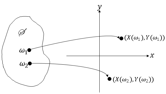
How do we define two random variables X,Y on a probability space (S,F,P)?
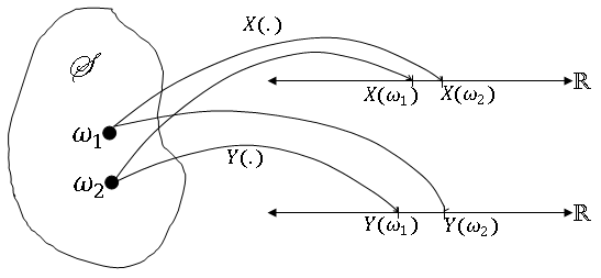
So two random variables can be viewed aw a mapping from S to R$ ^2 $, and (X,Y) is an ordered pair in R$ ^2 $. Note that we could draw the picture this way:
but this would not capture the joint behavior of X and Y. Note also that if X and Y are defined on two different probability spaces, those two spaces can be combined to create (S,F,P).
In order for X and Y to be a valid random variable pair, we will need to consider regions D ⊂ R$ ^2 $.
We need {(X,Y) ∈ O} ∈ F for any open rectangle O ⊂ R$ ^2 $, then {(X,Y) ∈ D} ∈ F ∀D ∈ B(R$ ^2 $).
But (X($ \omega $),Y($ \omega $)) ∈ O if X($ \omega $) ∈ A and Y($ \omega $) ∈ B for some A, B ∈ B(R), so {(X,Y) ∈ O} = X$ ^{-1} $(A) ∩ Y$ ^{-1} $(B)
If X and Y are valid random variables then
So,
So how do we find P((X,Y) ∈ D) for D ∈ B(R$ ^2 $)?
We will use joint cdfs, pdfs, and pmfs.
Joint Cumulative Distribution Function
Knowledge of F$ _X $(x) and F$ _Y $(y) alone will not be sufficient to compute P((X,Y) ∈ D) ∀D ∈ B(R$ ^2 $), in general.
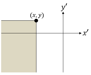
Definition $ \qquad $ The joint cumulative distribution function of random variables X,Y defined on (S,F,P) is F$ _{XY} $(x,y) ≡ P({X ≤ x} ∩ {Y ≤ y}) for x,y ∈ R.
Note that in this case, D ≡ D$ _{XY} $ = {(x',y') ∈ R$ ^2 $: x' ≤ x, y' ≤ y}
Properties of F$ _{XY} $:
$ \bullet\lim_{x\rightarrow -\infty}F_{XY}(x,y) = \lim_{y\rightarrow -\infty}F_{XY}(x,y) = 0 $
$ \begin{align} \bullet &\lim_{x\rightarrow \infty}F_{XY}(x,y) = F_Y(y)\qquad \forall y\in\mathbb R \\ &\lim_{y\rightarrow \infty}F_{XY}(x,y) = F_X(x)\qquad \forall x\in\mathbb R \end{align} $
F$ _X $ and F$ _Y $ are called the marginal cdfs of X and Y.
$ \bullet P(\{x_1 < X\leq x_2\}\cap\{y_1<Y\leq y_2\}) = F_{XY}(x_2,y_2)-F_{XY}(x_1,y_2)-F_{XY}(x_2,y_1)+F_{XY}(x_1,y_1) $
The Joint Probability Density Function
Definition $ \qquad $ The joint probability density function of random variables X and Y is
∀(x,y) ∈ R$ ^2 $ where the derivative exists.
It can be shown that if D ∈ B(R$ ^2 $), then,
where D ≡ D$ _{XY} $ = {(x',y') ∈ R$ ^2 $: x' ≤ x, y' ≤ y}
Properties of f$ _{XY} $:
$ \bullet f_{XY}(x,y)\geq 0\qquad\forall x,y\in\mathbb R $
$ \bullet \int\int_{\mathbb R}f_{XY}(x,y)dxdy = 1 $
$ \bullet F_{XY}(x,y) = \int_{-\infty}^{y}\int_{-\infty}^xf_{XY}(x',y')dx'dy'\qquad\forall(x,y)\in\mathbb R^2 $
$ \begin{align} \bullet &f_X(x) = \int_{-\infty}^{\infty}f_{XY}(x,y)dy \\ &f_Y(y) = \int_{-\infty}^{\infty}f_{XY}(x,y)dx \end{align} $ are the marginal pdfs of X and Y.
The Joint Probability Mass Function
If X and Y are discrete random variables, we will use the joint pdf given by
Note that if X is continuous and Y discrete (or vice versa), we will be interested in
We often use a form of Bayes' Theorem, which we will discuss later, to get this probability.
Joint Gaussian Random Variables
An important case of two random variables is: X and Y are jointly Gaussian if their joint pdf is given by
where μ$ _X $, μ$ _Y $, σ$ _X $, σ$ _Y $, r ∈ R; σ$ _X $,σ$ _Y $ > 0; -1 <r <1.
It can be shown that is X and Y are jointly Gaussian then X is N(μ$ _X $, σ$ _X $$ ^2 $) and Y is N(μ$ _Y $, σ$ _Y $$ ^2 $) (proof)
Special Case
We often model X and Y as jointly Gaussian with μ$ _X $ = μ$ _Y $ = 0, σ$ _X $ = σ$ _Y $ = σ, r = 0, so that
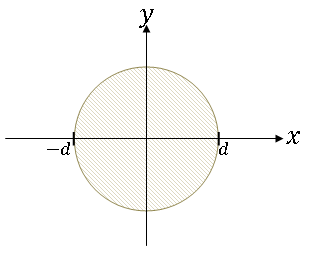
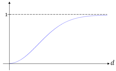
Example $ \qquad $ Let X and Y be jointly Gaussian with μ$ _X $ = μ$ _Y $ = 0, σ$ _X $ = σ$ _Y $ = σ, r = 0. Find the probability that (X,Y) lies within a distance d from the origin.
Let
Then
Use polar coordinates to make integration easier: let
Then
So the probability that (X,Y) lies within distance d from the origin looks like the graph in figure 5 (as a function of d).
References
- M. Comer. ECE 600. Class Lecture. Random Variables and Signals. Faculty of Electrical Engineering, Purdue University. Fall 2013.
Questions and comments
If you have any questions, comments, etc. please post them on this page

