| (6 intermediate revisions by 3 users not shown) | |||
| Line 1: | Line 1: | ||
| + | [[Category:slecture]] | ||
| + | [[Category:ECE438Fall2014Boutin]] | ||
| + | [[Category:ECE]] | ||
| + | [[Category:ECE438]] | ||
| + | [[Category:signal processing]] | ||
| + | [[Category:Discrete-time_Fourier_transform]] | ||
| + | |||
| + | |||
<center> | <center> | ||
<font size="4">DTFT of a Cosine Signal Sampled Above and Below the Nyquist Frequency </font> | <font size="4">DTFT of a Cosine Signal Sampled Above and Below the Nyquist Frequency </font> | ||
| Line 9: | Line 17: | ||
---- | ---- | ||
| + | |||
| + | |||
| + | <font size="4">Outline</font> | ||
| + | |||
| + | <font size="3"> | ||
| + | <ul> | ||
| + | <li> Introduction | ||
| + | <li> Sampling Above Nyquist Frequency </li> | ||
| + | <li> Sampling Below Nyquist Frequency </li> | ||
| + | <li> Conclusion </li> | ||
| + | </ul> | ||
| + | </font> | ||
| + | |||
| + | |||
| + | |||
| + | ---- | ||
| + | |||
| + | |||
| + | <font size="4">Introduction</font> | ||
| + | |||
<font size = '3'> | <font size = '3'> | ||
| Line 14: | Line 42: | ||
| − | |||
Lets look at a pure tone frequency F4 = 349Hz | Lets look at a pure tone frequency F4 = 349Hz | ||
| − | We will represent this tone as a cosine signal, <math>cos | + | We will represent this tone as a cosine signal, <math>cos(2\pi349t)</math> |
---- | ---- | ||
| + | |||
| + | |||
<font size="4">Sampling <u>Above</u> Nyquist Frequency</font> | <font size="4">Sampling <u>Above</u> Nyquist Frequency</font> | ||
| Line 69: | Line 98: | ||
The frequency content of the original signal lies within the -<math>\pi</math> to <math>\pi </math> band. Therefore the signal can be properly reconstructed. | The frequency content of the original signal lies within the -<math>\pi</math> to <math>\pi </math> band. Therefore the signal can be properly reconstructed. | ||
| + | |||
| + | |||
| + | |||
| + | ---- | ||
| + | |||
<font size="4">Sampling <u>Below</u> Nyquist Frequency</font> | <font size="4">Sampling <u>Below</u> Nyquist Frequency</font> | ||
| Line 106: | Line 140: | ||
&= rep_{2\pi}\pi (\delta(\omega - 2\pi\frac{349}{500}) + \delta(\omega + 2\pi\frac{349}{500})) \\ | &= rep_{2\pi}\pi (\delta(\omega - 2\pi\frac{349}{500}) + \delta(\omega + 2\pi\frac{349}{500})) \\ | ||
| − | &= rep_{2\pi}\frac{500}{2} ((\delta(\frac{500}{2\pi}\omega - | + | &= rep_{2\pi}\frac{500}{2} ((\delta(\frac{500}{2\pi}\omega - 349) + \delta(\frac{500}{2\pi}\omega + 349)) \\ |
\end{align} | \end{align} | ||
</math> | </math> | ||
| + | |||
| + | Use periodicity property of cosine to shift from -<math>2\pi</math> to <math>2\pi </math> to -<math>\pi</math> to <math>\pi </math> band. | ||
| + | |||
| + | <math>X_{1}(\omega) = rep_{2\pi}\frac{500}{2} ((\delta(\frac{500}{2\pi}\omega - 151) + \delta(\frac{500}{2\pi}\omega + 151)) </math> | ||
Plot of <math>X_{2}(\omega)</math>: | Plot of <math>X_{2}(\omega)</math>: | ||
| Line 116: | Line 154: | ||
As you can see the original signal frequency exists outside of the -<math>\pi</math> to <math>\pi </math> band. | As you can see the original signal frequency exists outside of the -<math>\pi</math> to <math>\pi </math> band. | ||
The frequencies that exists within this band are copies of the original signal that are 'rep'ed. Therefore these frequencies do not represent the frequency content of the the original signal, resulting in aliasing. | The frequencies that exists within this band are copies of the original signal that are 'rep'ed. Therefore these frequencies do not represent the frequency content of the the original signal, resulting in aliasing. | ||
| + | |||
| + | |||
| + | ---- | ||
| + | |||
| + | <font size ="4"> | ||
| + | Conclusion | ||
| + | |||
| + | <font size="3"> | ||
| + | When sampling above the Nyquist frequency the signal can be accurately represented but when sampling below the signal will become aliased. | ||
| + | |||
| + | |||
| + | |||
| + | [[DTFTCosinePawlingQuestions| Questions and Comments]] | ||
| + | ---- | ||
| + | [[2014_Fall_ECE_438_Boutin_digital_signal_processing_slectures|Back to ECE438 slectures, Fall 2014]] | ||
Latest revision as of 20:04, 16 March 2015
DTFT of a Cosine Signal Sampled Above and Below the Nyquist Frequency
A slecture by ECE student Andrew Pawling
Partly based on the ECE438 Fall 2014 lecture material of Prof. Mireille Boutin.
Outline
- Introduction
- Sampling Above Nyquist Frequency
- Sampling Below Nyquist Frequency
- Conclusion
Introduction
In this slecture we will look at an example that illustrates the Nyquist condition. When a signal is sampled, frequencies above half the sampling rate cannot be properly represented and result in aliasing.
Lets look at a pure tone frequency F4 = 349Hz
We will represent this tone as a cosine signal, $ cos(2\pi349t) $
Sampling Above Nyquist Frequency
For this signal $ f_{s} > 2f_{m} = 2(349)Hz = 698Hz $ or else aliasing will occur. We will choose a sampling frequency of $ f_{s} = 1/T_{1} = 1000Hz $.
$ \begin{align} x_{1}(n) &= x(nT_{1}) \\ &= cos(2\pi349nT_{1}) \\ &= cos(\frac{2\pi349n}{1000}) \\ &= \frac{1}{2}(e^{\frac{-j2\pi349n}{1000}} + e^{\frac{j2\pi349n}{1000}}) \\ \\ \\ \end{align} $
$ Note\ that:\ 0 < |\pm2\pi\frac{349}{1000}| < \pi $
This means the original signal can be properly represented when sampled at $ f_{s} = 1000Hz. $
Using the discrete-time Fourier transform pair for cosine:
$ x[n] \ \ \ \ \ \ \ \ \ \ -----> \ \ \ \ X(\omega) $
$ cos(\omega_{0}n) \ \ \ \ -----> \ \ \ \ \pi\sum_{k=-\infty}^\infty (\delta(\omega -\omega_{0}+2\pi k) + \delta(\omega + \omega_{0}+2\pi k)) $
$ \begin{align} X_{1}(\omega) &= \pi \sum_{k=-\infty}^\infty(\delta(\omega - 2\pi\frac{349}{1000} +2\pi k) + \delta(\omega + 2\pi\frac{349}{1000} + 2\pi k)) \\ &= rep_{2\pi}\pi (\delta(\omega - 2\pi\frac{349}{1000}) + \delta(\omega + 2\pi\frac{349}{1000})) \\ &= rep_{2\pi}\frac{1000}{2} ((\delta(\frac{1000}{2\pi}\omega - 349) + \delta(\frac{1000}{2\pi}\omega + 349)) \\ \end{align} $
Plot of $ X_{1}(\omega) $:
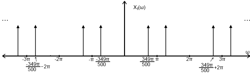 Repeats every $ 2\pi $
The frequency content of the original signal lies within the -$ \pi $ to $ \pi $ band. Therefore the signal can be properly reconstructed.
Sampling Below Nyquist Frequency
For this signal $ f_{s} > 2f_{m} = 2(349)Hz = 698Hz $ or else aliasing will occur. We will choose a sampling frequency that does not satisfy this condition this time. Let's use $ f_{s} = 1/T_{2} = 500Hz $.
$ \begin{align} x_{2}(n) &= x(nT_{2}) \\ &= cos(2\pi349nT_{2}) \\ &= cos(\frac{2\pi349n}{500}) \\ &= \frac{1}{2}(e^{\frac{-j2\pi349n}{500}} + e^{\frac{j2\pi349n}{500}}) \\ \\ \\ \end{align} $
$ Note\ that:\ \pi < |\pm2\pi\frac{349}{500}| < 2\pi $
This means the original signal cannot be properly represented when sampled at $ f_{s} = 500Hz. $
Using the discrete-time Fourier transform pair for cosine again:
$ x[n] \ \ \ \ \ \ \ \ \ \ -----> \ \ \ \ X(\omega) $
$ cos(\omega_{0}n) \ \ \ \ -----> \ \ \ \ \pi\sum_{k=-\infty}^\infty (\delta(\omega -\omega_{0}+2\pi k) + \delta(\omega + \omega_{0}+2\pi k)) $
$ \begin{align} X_{1}(\omega) &= \pi \sum_{k=-\infty}^\infty(\delta(\omega - 2\pi\frac{349}{500} +2\pi k) + \delta(\omega + 2\pi\frac{349}{500} + 2\pi k)) \\ &= rep_{2\pi}\pi (\delta(\omega - 2\pi\frac{349}{500}) + \delta(\omega + 2\pi\frac{349}{500})) \\ &= rep_{2\pi}\frac{500}{2} ((\delta(\frac{500}{2\pi}\omega - 349) + \delta(\frac{500}{2\pi}\omega + 349)) \\ \end{align} $
Use periodicity property of cosine to shift from -$ 2\pi $ to $ 2\pi $ to -$ \pi $ to $ \pi $ band.
$ X_{1}(\omega) = rep_{2\pi}\frac{500}{2} ((\delta(\frac{500}{2\pi}\omega - 151) + \delta(\frac{500}{2\pi}\omega + 151)) $
Plot of $ X_{2}(\omega) $:
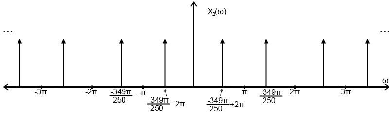
As you can see the original signal frequency exists outside of the -$ \pi $ to $ \pi $ band. The frequencies that exists within this band are copies of the original signal that are 'rep'ed. Therefore these frequencies do not represent the frequency content of the the original signal, resulting in aliasing.
Conclusion
When sampling above the Nyquist frequency the signal can be accurately represented but when sampling below the signal will become aliased.
