Nearest Neighbor Method
A slecture by student Sang Ho Yoon
Partly based on the ECE662 Spring 2014 lecture material of Prof. Mireille Boutin.
Contents
[hide]Introduction
In this slecture, basic principles of implementing nearest neighbor rule will be covered. The error related to the nearest neighbor rule will be discussed in detail including convergence, error rate, and error bound. Since the nearest neighbor rule relies on metric function between patterns, the properties of metrics will be studied in detail. Example of different metrics will be introduced with its characteristics. The representative of real application such as body posture recognition using Procrustes metric could be a good example to understand the nearest neighbor rule.----
Nearest Neighbor Basic Principle
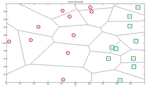
Let's consider a testing sample x. Based on labeled training sample $ D^n = x_{1},... ,x_{n}, $ the nearest neighbor technique will find the closest point x' to x. Then we assign the class of x' to x. This is how the classification based on the nearest neighbor rule is processed. Although this rule is very simple, it is also reasonable. The label $ \theta' $ used in the nearest neighbor is random variable which means $ \theta' = w_{i} $ is same as a posteriori probability $ P(w_{i}|x'). $ If sample sizes are big enough, it could be assumed that x' is sufficiently close to x that $ P(w_{i}|x') = P(w_{i}|x). $ Using the nearest neighbor rule, we could get high accuracy classification if sample sizes are guaranteed. In other words, the nearest neighbor rule is matching perfectly with probabilities in nature.

Error Rate & Bound using NN
In order to find the error rate and bound related to the nearest neighbor rule, we need to confirm the convergence of the nearest neighbor as sample increases to the infinity. We set $ P = \lim_{n \to \infty}P_n(e) $. Then, we set infinite sample conditional average probability of error as $ P(e|x) $. Using this the unconditional average probability of error which indicates the average error according to training samples can be shown as
Since minimum error caused by the nearest neighbor cannot be lower than error from Bayes decision rule, the minimum possible value of the error $ P^*(e|x) $ can be represented as
In real application, we cannot guarantee that sufficient number of samples are used for training. In some cases, small sample sizes could lead to an accidental characteristics where it will eventually lead to an error. The decision will be made on based on this nearest neighbor which introduces a conditional probability error $ P(e|x,x') $. Again, averaging over x', we will get
Above equation, however, becomes trivial since $ p(x|x') $ forms a delta function centered at x. This condition gives out the positive number $ P_s $ which is the probability that any sample falls within a hypersphere $ \mathbb{S} $ centered about x
This means that the probability that independently drawn samples fall outside of hypersphere $ \mathbb{S} $ is $ (1-P_s)^n $. This equation will approach zero as n goes to infinity. This proves that x' converges to x with infinite number of samples.
The proof of the convergence of the nearest neighbor rule ensures that the error rate could be theoretically formulated. The conditional probability of error $ P_n(e|x,x') $ can be utilized to form theoretical error rate. Let's assume $ x'_n $ is nearest neighbor where n indicates number of samples. Now we have,
Using the nearest neighbor rule, the error occurs when $ \theta \neq \theta'_n $. This will bring following conditional probability of error.
The asymptotic nearest neighbor error rate will be formulated by using previous equation and exchange some limits and integrals.
Previously, it was mentioned that the nearest neighbor cannot be better than Bayes decision. Therefore, it will be intuitive to represent the error bound of NN rule in terms of Bayes rate $ P^* $. Since Bayes rate is a minimum possible error we could obtain, the lower error bound should be fixed to $ P^* $. The upper bound, however, will change according to given $ P^* $. The exact error rate obtained in previous section can be utilized to get the upper error bound. First we set
with following two constraints and utilize these with above equation will introduce new equation.
- $ P(w_i|x) \geq 0 $
- $ \sum_{i\neq m}P(w_i|x)=1-P(w_m|x)=P^*(e|x) $
These will lead to following inequalities.
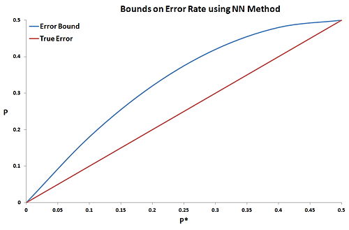
This clearly demonstrates that the nearest neighbor rule's maximum error rate is less than twice of Bayes decision error ($ P \leq 2P^* $). Obviously we can get better error bound by observing the variance where
Applying this equation with previous equation, we will get the desired error bounds on the nearest neighbor rule for infinite number of samples. Figure 2 illustrates the graphical error bound of the nearest neighbor rule based on above equations.

Metrics Type & Application
However, the closest distance between x' and x is determined by which metrics are used for feature space. A "metric" on a space S is a function which has following 4 properties:
- Non-negativity : $ D(\vec{x_{1}},\vec{x_{2}}) \geq 0, \forall \vec{x_{1}},\vec{x_{2}} \in S $
- Symmetry : $ D(\vec{x_{1}},\vec{x_{2}}) = D(\vec{x_{2}},\vec{x_{1}}), \forall \vec{x_{1}},\vec{x_{2}} \in S $
- Reflexivity : $ D(\vec{x},\vec{x}) = 0, \forall \vec{x} \in S $
- Triangle Inequality : $ D(\vec{x_{1}},\vec{x_{2}}) + D(\vec{x_{2}},\vec{x_{3}}) \geq D(\vec{x_{1}},\vec{x_{3}}), \forall \vec{x_{1}},\vec{x_{2}},\vec{x_{3}} \in S $
There are many metrics which satisfy above properties. The example metrics are followings:
- Euclidean distance: $ D(\vec{x_1},\vec{x_2})=||\vec{x_1}-\vec{x_2}||_{L_2}=\sqrt{\sum_{i=1}^n ({x_1}^i-{x_2}^i)^2} $
- Manhattan (cab driver) distance: $ D(\vec{x_1},\vec{x_2})=||\vec{x_1}-\vec{x_2}||_{L_1}=\sum_{i=1}^n |{x_1}^i-{x_2}^i| $
- Minkowski metric: $ D(\vec{x_1},\vec{x_2})=||\vec{x_1}-\vec{x_2}||_{L_p}=(\sum_{i=1}^n ({x_1}^i-{x_2}^i)^p)^{\frac{1}{p}} $
- Riemannian metric: $ D(\vec{x_1},\vec{x_2}) = \sqrt{(\vec{x_1}-\vec{x_2})^\top \mathbb{M}(\vec{x_1}-\vec{x_2})} $
- Infinite norm: $ D(\vec{x_1},\vec{x_2})=||\vec{x_1}-\vec{x_2}||_{\infty}=max_i |{x_1}^i-{x_2}^i| $
Since these different metrics share common properties, the dissection areas are almost similar. However, the different distance calculation makes the shape of the boundary different from each other. For problem with two features with no similarity, the Tanimoto metric is widely used. The Tanimoto concentrates on calculating the distance between two sets as
In here $ n_1 $ and $ n_2 $ represent number of elements in the set and $ n_{12} $ means the number of common elements in both sets. Let's consider following example,
$ n_1=\{fever, skinrash, high blood pressure\} $
$ n_2=\{fever, neck stiffness\} $
In this case $ n_1 = 3, n_2 =2 $, and $ n_{12} = 1 $.
Use of different metrics enhances an accuracy of the nearest neighbor rule for several applications. The body recognition is one of the main application of the nearest neighbor rule. The body posture recognition is very complex since the coordinates varies even with same posture due to translation and rotation. Adopting conventional Euclidean distance will not identify same posture with different translation and rotation. Before comparing the actual posture, testing sample should be translated and rotated inversely to the training sample for right comparison of each point. Procrustes metric will approach the problem with the translation and rotation compensation. Following equation describes how Procrustes metric works
$ p=(p_1, p_2, \cdots ,p_N),\bar p = (\bar p_1, \bar p_2, \cdots ,\bar p_N) $
$ p $ indicates testing sample while $ \bar p $ refers single instance of training sample. As you can see, the compensation on rotation and translation has been before comparing the distance between testing sample and training sample. Alternative approach is also available where we use invariant coordinates as feature vectors. The invariant coordinates do not change under translation and rotation effect. In other words, find $ \varphi $ such that
$ \varphi (x) = \varphi(\vec{x}) $
Typical example of the invariant coordinates of the body can be the distance between fixed joints. Let's consider simple 1D problem where we count distance as invariant coordinates. In this example, our feature vectors are distance and we only compare the distance for the classification.
Figure 3 illustrates the use of the nearest neighbor method for shape searching. Adopting special metrics introduced previously, the robust and low-cost classifier could be set. However, users always have to be cautious on choosing invariant coordinates. For instance, the distance is not a feature vector that always works. Thus, we should select proper feature vectors which are invariant during specific situation. There are timebased, geometric, and dimensionless geometric invariants which could be utilized in the application.

Discussion
In this lecture we go over from basic principle of the nearest neighbor rule to its application. Throughout the lecture, the error rate and error bound is found out that the minimum error cannot be lower than Bayes error and the maximum error cannot be bigger than twice of Bayes error. With the sufficient sample sizes, it is reasonable to use the nearest neighbor for the classification. The study of the different metrics show that various metrics are available for specific need from each application. The example of posture recognition using the nearest neighbor demonstrates that proper metric adoption is critical to enhance the classification result. Use of proper metric with the nearest neighbor classification will result in forming reasonable classifier.
References
$ [1] $ Pattern classification. Richard O. Duda, Peter E. Hart, and David G. Stork.
$ [2] $ Invariant signature-based modeling, classification and estimation Lecture, http://www.mech.kuleuven.be/en/pma/research/robotics/research/invariants
$ [3] $ Northwestern pattern recognition e-lecture, http://users.eecs.northwestern.edu/~yingwu/teaching/EECS510/Notes/NearestNeighbor_1_handout.pdf
$ [4] $ Introduction to Statistical Pattern Recognition. K. Fukunaga.
$ [5] $ Lecture notes from ECE662: Statistical Pattern Recognition and Decision Making Processes, Purdue University, Mireille Boutin
$ [6] $ Elena Deza & Michel Marie Deza (2009) Encyclopedia of Distances, page 94, Springer.
Questions and comments
If you have any questions, comments, etc. please post them on this page.

