| Line 11: | Line 11: | ||
== Continuity at a point== | == Continuity at a point== | ||
| − | Let's consider the the following three functions along with their graphs (in blue). The red dots in each correspond to <math>x=0</math>, e.g. for <math> | + | Let's consider the the following three functions along with their graphs (in blue). The red dots in each correspond to <math>x=0</math>, e.g. for <math>f_1</math>, the red dot is the point <math>(0,f_1(0))=(0,0)</math>. Ignore the red dashed lines for now; we will explain them later. |
| − | :<math>\displaystyle | + | :<math>\displaystyle f_1(x)=x^3</math> |
[[Image:limits_of_functions_f.png]] | [[Image:limits_of_functions_f.png]] | ||
| − | :<math> | + | :<math>f_2(x)=\begin{cases}-x^2-\frac{1}{2} &\text{if}~x<0\\ x^2+\frac{1}{2} &\text{if}~x\geq 0\end{cases}</math> |
[[Image:limits_of_functions_g.png]] | [[Image:limits_of_functions_g.png]] | ||
| − | :<math> | + | :<math>f_3(x)=\begin{cases} \sin\left(\frac{1}{x}\right) &\text{if}~x\neq 0\\ 0 &\text{if}~x=0\end{cases}</math> |
[[Image:limits_of_functions_h.png]] | [[Image:limits_of_functions_h.png]] | ||
| − | We can see from the graphs that <math> | + | We can see from the graphs that <math>f_1</math> is "continuous" at <math>0</math>, and that <math>f_2</math> and <math>f_3</math> are "discontinuous" at 0. But, what exactly do we mean? Intuitively, <math>f_1</math> seems to be continuous at <math> 0</math> because <math>f_1(x)</math> is close to <math>f_1(0)</math> whenever <math>x</math> is close to <math> 0</math>. On the other hand, <math>f_2</math> appears to be discontinuous at <math> 0</math> because there are points <math>x</math> which are close to <math>0</math> but such that <math>f_2(x)</math> is far away from <math>f_2(0)</math>. The same observation applies to <math>f_3</math>. |
| − | Let's make these observations more precise. First, we will try to estimate <math> | + | Let's make these observations more precise. First, we will try to estimate <math>f_1(0)</math> with error at most <math>0.25</math>, say. In the graph of <math>f_1</math>, we have marked off a band of width <math>0.5</math> about <math>f_1(0)</math>. So, any point in the band will provide a good approximation here. As a first try, we might think that if <math>x</math> is close enough to <math>0</math>, then <math>f_1(x)</math> will be a good estimate of <math>f_1(0)</math>. Indeed, we see from the graph that for ''any'' <math>x</math> in the interval <math>(-\sqrt[3]{0.25},\sqrt[3]{0.25})</math>, <math>f_1(x)</math> lies in the band (or if we wish to be more pedantic, we would say that <math>(x,f_1(x))</math> lies in the band). So, "close enough to <math>0</math>" here means in the interval <math>(-\sqrt[3]{0.25},\sqrt[3]{0.25})</math>; note that ''any'' point which is close enough to <math>0</math> provides a good approximation of <math>f_1(0)</math>. |
| − | There is nothing special about our error bound <math>0.25</math>. Choose a positive number <math>\varepsilon</math>, and suppose we would like to estimate <math> | + | There is nothing special about our error bound <math>0.25</math>. Choose a positive number <math>\varepsilon</math>, and suppose we would like to estimate <math>f_1(0)</math> with error at most <math>\varepsilon</math>. Then, as above, we can find some interval <math>\displaystyle(-\delta,\delta)</math> about <math>0</math> (if you like to be concrete, any <math>\displaystyle\delta</math> such that <math>0<\delta<\sqrt[3]{\varepsilon}</math> will do) such that <math>f_1(x)</math> is a good estimate for <math>f_1(0)</math> for ''any'' <math>x</math> in <math>\displaystyle(-\delta,\delta)</math>. In other words, for ''any'' <math>x</math> which is close enough to <math>0</math>, <math>f_1(x)</math> will be no more than <math>\varepsilon</math> away from <math>f_1(0)</math>. |
| − | Can we do the same for <math> | + | Can we do the same for <math>f_2</math>? That is, if <math>x</math> is close enough to <math>0</math>, then will <math>f_2(x)</math> be a good estimate of <math>f_2(0)</math>? Well, we see from the graph that <math>f_2(0.25)</math> provides a good approximation to <math>f_2(0)</math>. But if <math>0.25</math> is close enough to <math>0</math>, then certainly <math>-0.25</math> should be too; however, the graph shows that <math>f_2(-0.25)</math> is not a good estimate of <math>f_2(0)</math>. In fact, for any <math>x>0</math>, <math>f_2(-x)</math> will never be a good approximation for <math>f_2(0)</math>, even though <math>x</math> and <math>-x</math> are the same distance from <math>0</math>. |
| − | In contrast to <math> | + | In contrast to <math>f_1</math>, we see that for any interval <math>\displaystyle(-\delta,\delta)</math> about <math>0</math>, we can find an <math>x</math> in <math>\displaystyle(-\delta,\delta)</math> such that <math>f_2(x)</math> is more than <math>0.25</math> away from <math>f_2(0)</math>. |
| − | The same is true for <math> | + | The same is true for <math>f_3</math>. Whenever we find an <math>x</math> such that <math>f_3(x)</math> lies in the band, we can always find a point <math>y</math> such that 1) <math>y</math> is just as close or closer to <math>0</math> and 2) <math>f_3(y)</math> lies outside the band. So, it is not true that if <math>x</math> is close enough to <math>0</math>, then <math>f_3(x)</math> will be a good estimate for <math>f_3(0)</math>. |
| − | Let's summarize what we have found. For <math> | + | Let's summarize what we have found. For <math>f_1</math>, we saw that for each <math>\varepsilon>0</math>, we can find an interval <math>\displaystyle(-\delta,\delta)</math> about <math>0</math> (<math>\displaystyle\delta</math> depends on <math>\varepsilon</math>) so that for every <math>x</math> in <math>\displaystyle(-\delta,\delta)</math>, <math>|f_1(x)-f_1(0)|<\varepsilon</math>. However, <math>f_2</math> does not satisfy this property. More specifically, there is an <math>\varepsilon>0</math>, namely <math>\varepsilon=0.25</math>, so that for any interval <math>\displaystyle(-\delta,\delta)</math> about <math>0</math>, we can find an <math>x</math> in <math>\displaystyle(-\delta,\delta)</math> such that <math>|f_2(x)-f_2(0)|\geq\varepsilon</math>. The same is true of <math>f_3</math>. |
Now we state the formal definition of continuity at a point. Compare this carefully with the previous paragraph. | Now we state the formal definition of continuity at a point. Compare this carefully with the previous paragraph. | ||
| Line 43: | Line 43: | ||
== The Limit of a Function at a Point == | == The Limit of a Function at a Point == | ||
| − | Now, let's consider the two functions <math> | + | Now, let's consider the two functions <math>g_1</math> and <math>g_2</math> below. Note that <math>F</math> is left undefined at <math>0</math>. |
| − | :<math> | + | :<math>g_1(x)=\begin{cases}-x^2-x &\text{if}~x<0\\ x&\text{if}~x>0\end{cases}</math> |
[[Image:limits_of_functions_f2.png]] | [[Image:limits_of_functions_f2.png]] | ||
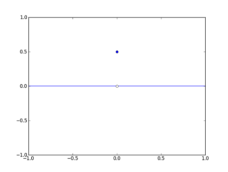
| − | :<math> | + | :<math>g_2(x)=\begin{cases}0 &\text{if}~x\neq 0\\ \frac{1}{2}&\text{if}~x=0\end{cases}</math> |
[[Image:limits_of_functions_g2.png]] | [[Image:limits_of_functions_g2.png]] | ||
| − | Recall the function <math> | + | Recall the function <math>f_1</math> from the previous section. We found that it was continuous at <math>0</math> because <math>f_1(x)</math> is close to <math>f_1(0)</math> if <math>x</math> is close enough to <math>0</math>. We can do something similar with <math>g_1</math> and <math>g_2</math> here. From the graph, we can see that <math>g_1(x)</math> is close to <math>0</math> whenever <math>x</math> is close enough, but not equal to, <math>0</math>. Similarly, we see that <math>g_2(x)</math> is close to <math>0</math> whenever <math>x</math> is close enough, but not equal to, <math>0</math>. The "not equal" part is important for both <math>g_1</math> and <math>g_2</math> because <math>g_1</math> is undefined at <math>x=0</math> while <math>g_2</math> has a discontinuity there. The idea here is similar to that of continuity, but we ignore whatever happens at <math>x=0</math>. We are concerned more with how <math>g_1</math> and <math>g_2</math> behave near <math>0</math> rather than at <math>0</math>. This leads to the following definition. |
| − | '''DEFINITION.''' Let <math>f</math> be a function defined for all real numbers, with possibly one exception, and with range <math>\mathbb{R}</math>. Let <math>c</math> be any real number. We say that the limit of <math>f</math> at <math>c</math> is <math>b</math> and write <math>\lim_{x\to c}f(x)=b</math> if for every <math>\varepsilon>0</math>, there is a <math>\displaystyle\delta>0</math> such that <math>|f(x)-b|<\varepsilon</math> whenever <math>\displaystyle 0<|x-c|<\delta</math>. | + | '''DEFINITION.''' Let <math>f</math> be a function defined for all real numbers, with possibly one exception, and with range <math>\mathbb{R}</math>. Let <math>c</math> be any real number. We say that the limit of <math>f</math> at <math>c</math> is <math>b</math>, or that the limit of <math>f(x)</math> as <math>x</math> approaches <math>c</math> is <math>b</math>, and write <math>\lim_{x\to c}f(x)=b</math> if for every <math>\varepsilon>0</math>, there is a <math>\displaystyle\delta>0</math> such that <math>|f(x)-b|<\varepsilon</math> whenever <math>\displaystyle 0<|x-c|<\delta</math>. |
| − | This is the same as the definition for continuity, except we ignore what happens at <math>c</math>. We can see this in two places in the above definition. The first is the use of <math>b</math> instead of <math>f(c)</math>, and the second is the condition <math>\displaystyle 0<|x-c|<\delta</math>, which says that <math>x</math> is close enough, but not equal to, <math>c</math>. | + | This is the same as the definition for continuity, except we ignore what happens at <math>c</math>. We can see this in two places in the above definition. The first is the use of <math>b</math> instead of <math>f(c)</math>, and the second is the condition <math>\displaystyle 0<|x-c|<\delta</math>, which says that <math>x</math> is close enough, but not equal to, <math>c</math>. The restriction on the domain of <math>f</math> in the above definition is not really necessary; if <math>f</math> has domain <math>A\subset\mathbb{R}</math>, we can define <math>\lim_{x\to c}f(x)</math> for any <math>c</math> which is a "limit point" of <math>\displaystyle A</math>. But, in calculus, one usually encounters the situation described in the definition. |
| − | + | If you've ever seen "Mean Girls," you know that the limit does not always exist. For example, if <math>f_2</math> is the function in the previous section, then <math>\lim_{x\to 0}f_2(x)</math> does not exist. We will show this rigorously in the exercises, but it is clear from the graph of <math>f_2</math>. | |
| + | |||
| + | Having defined what a limit is, we can now look at the relationship between continuity and limit. As a first step, we can now restate the definition of continuity at a point more succinctly in terms of limits: <math>f</math> is continuous at <math>c</math> if and only if <math>\displaystyle\lim_{x\to c}f(x)=f(c)</math>. Now, let's take a look at the functions <math>g_1</math> and <math>g_2</math> defined earlier. | ||
---- | ---- | ||
Revision as of 01:48, 12 May 2014
Contents
[hide]Limit of a Function at a Point
by: Michael Yeh, proud Member of the Math Squad.
keyword: tutorial, limit, function, sequence
INTRODUCTION
Provided here is a brief introduction to the concept of "limit," which features prominently in calculus. We first discuss the limit of a function at a point; to help motivate the definition, we first consider continuity at a point. Unless otherwise mentioned, all functions here will have domain and range $ \mathbb{R} $, the real numbers. Words such as "all," "every," "each," "some," and "there is/are" are quite important here; read carefully!
Continuity at a point
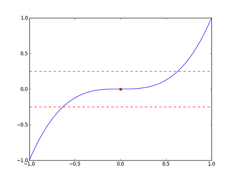
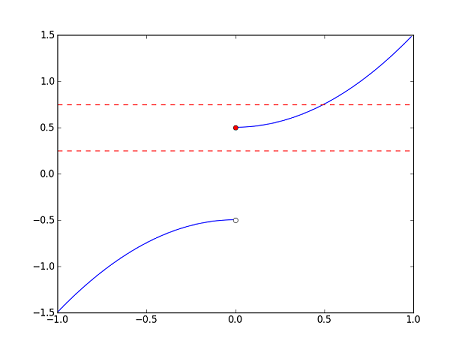
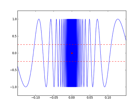
Let's consider the the following three functions along with their graphs (in blue). The red dots in each correspond to $ x=0 $, e.g. for $ f_1 $, the red dot is the point $ (0,f_1(0))=(0,0) $. Ignore the red dashed lines for now; we will explain them later.
- $ \displaystyle f_1(x)=x^3 $
- $ f_2(x)=\begin{cases}-x^2-\frac{1}{2} &\text{if}~x<0\\ x^2+\frac{1}{2} &\text{if}~x\geq 0\end{cases} $
- $ f_3(x)=\begin{cases} \sin\left(\frac{1}{x}\right) &\text{if}~x\neq 0\\ 0 &\text{if}~x=0\end{cases} $
We can see from the graphs that $ f_1 $ is "continuous" at $ 0 $, and that $ f_2 $ and $ f_3 $ are "discontinuous" at 0. But, what exactly do we mean? Intuitively, $ f_1 $ seems to be continuous at $ 0 $ because $ f_1(x) $ is close to $ f_1(0) $ whenever $ x $ is close to $ 0 $. On the other hand, $ f_2 $ appears to be discontinuous at $ 0 $ because there are points $ x $ which are close to $ 0 $ but such that $ f_2(x) $ is far away from $ f_2(0) $. The same observation applies to $ f_3 $.
Let's make these observations more precise. First, we will try to estimate $ f_1(0) $ with error at most $ 0.25 $, say. In the graph of $ f_1 $, we have marked off a band of width $ 0.5 $ about $ f_1(0) $. So, any point in the band will provide a good approximation here. As a first try, we might think that if $ x $ is close enough to $ 0 $, then $ f_1(x) $ will be a good estimate of $ f_1(0) $. Indeed, we see from the graph that for any $ x $ in the interval $ (-\sqrt[3]{0.25},\sqrt[3]{0.25}) $, $ f_1(x) $ lies in the band (or if we wish to be more pedantic, we would say that $ (x,f_1(x)) $ lies in the band). So, "close enough to $ 0 $" here means in the interval $ (-\sqrt[3]{0.25},\sqrt[3]{0.25}) $; note that any point which is close enough to $ 0 $ provides a good approximation of $ f_1(0) $.
There is nothing special about our error bound $ 0.25 $. Choose a positive number $ \varepsilon $, and suppose we would like to estimate $ f_1(0) $ with error at most $ \varepsilon $. Then, as above, we can find some interval $ \displaystyle(-\delta,\delta) $ about $ 0 $ (if you like to be concrete, any $ \displaystyle\delta $ such that $ 0<\delta<\sqrt[3]{\varepsilon} $ will do) such that $ f_1(x) $ is a good estimate for $ f_1(0) $ for any $ x $ in $ \displaystyle(-\delta,\delta) $. In other words, for any $ x $ which is close enough to $ 0 $, $ f_1(x) $ will be no more than $ \varepsilon $ away from $ f_1(0) $.
Can we do the same for $ f_2 $? That is, if $ x $ is close enough to $ 0 $, then will $ f_2(x) $ be a good estimate of $ f_2(0) $? Well, we see from the graph that $ f_2(0.25) $ provides a good approximation to $ f_2(0) $. But if $ 0.25 $ is close enough to $ 0 $, then certainly $ -0.25 $ should be too; however, the graph shows that $ f_2(-0.25) $ is not a good estimate of $ f_2(0) $. In fact, for any $ x>0 $, $ f_2(-x) $ will never be a good approximation for $ f_2(0) $, even though $ x $ and $ -x $ are the same distance from $ 0 $.
In contrast to $ f_1 $, we see that for any interval $ \displaystyle(-\delta,\delta) $ about $ 0 $, we can find an $ x $ in $ \displaystyle(-\delta,\delta) $ such that $ f_2(x) $ is more than $ 0.25 $ away from $ f_2(0) $.
The same is true for $ f_3 $. Whenever we find an $ x $ such that $ f_3(x) $ lies in the band, we can always find a point $ y $ such that 1) $ y $ is just as close or closer to $ 0 $ and 2) $ f_3(y) $ lies outside the band. So, it is not true that if $ x $ is close enough to $ 0 $, then $ f_3(x) $ will be a good estimate for $ f_3(0) $.
Let's summarize what we have found. For $ f_1 $, we saw that for each $ \varepsilon>0 $, we can find an interval $ \displaystyle(-\delta,\delta) $ about $ 0 $ ($ \displaystyle\delta $ depends on $ \varepsilon $) so that for every $ x $ in $ \displaystyle(-\delta,\delta) $, $ |f_1(x)-f_1(0)|<\varepsilon $. However, $ f_2 $ does not satisfy this property. More specifically, there is an $ \varepsilon>0 $, namely $ \varepsilon=0.25 $, so that for any interval $ \displaystyle(-\delta,\delta) $ about $ 0 $, we can find an $ x $ in $ \displaystyle(-\delta,\delta) $ such that $ |f_2(x)-f_2(0)|\geq\varepsilon $. The same is true of $ f_3 $.
Now we state the formal definition of continuity at a point. Compare this carefully with the previous paragraph.
DEFINITION. Let $ f $ be a function from $ \displaystyle A $ to $ \mathbb{R} $, where $ A\subset\mathbb{R} $. Then $ f $ is continuous at a point $ c\in A $ if for every $ \varepsilon>0 $, there is a $ \displaystyle\delta>0 $ such that $ |f(x)-f(c)|<\varepsilon $ for any $ x $ that satisfies $ \displaystyle|x-c|<\delta $. $ f $ is said to be continuous if it is continuous at every point of $ A $.
In our language above, $ \varepsilon $ is the error bound, and $ \displaystyle\delta $ is our measure of "close enough (to $ c $)." Note that continuity is defined only for points in a function's domain. So, the function $ k(x)=1/x $ is technically continuous because $ 0 $ is not in the domain of $ k $. If, however, we defined $ k(0)=0 $, then $ k $ will no longer be continuous.
The Limit of a Function at a Point
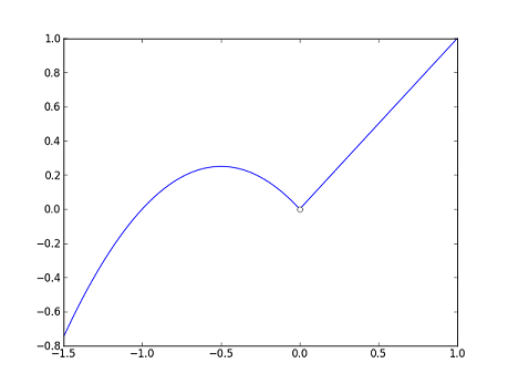
Now, let's consider the two functions $ g_1 $ and $ g_2 $ below. Note that $ F $ is left undefined at $ 0 $.
- $ g_1(x)=\begin{cases}-x^2-x &\text{if}~x<0\\ x&\text{if}~x>0\end{cases} $
- $ g_2(x)=\begin{cases}0 &\text{if}~x\neq 0\\ \frac{1}{2}&\text{if}~x=0\end{cases} $
Recall the function $ f_1 $ from the previous section. We found that it was continuous at $ 0 $ because $ f_1(x) $ is close to $ f_1(0) $ if $ x $ is close enough to $ 0 $. We can do something similar with $ g_1 $ and $ g_2 $ here. From the graph, we can see that $ g_1(x) $ is close to $ 0 $ whenever $ x $ is close enough, but not equal to, $ 0 $. Similarly, we see that $ g_2(x) $ is close to $ 0 $ whenever $ x $ is close enough, but not equal to, $ 0 $. The "not equal" part is important for both $ g_1 $ and $ g_2 $ because $ g_1 $ is undefined at $ x=0 $ while $ g_2 $ has a discontinuity there. The idea here is similar to that of continuity, but we ignore whatever happens at $ x=0 $. We are concerned more with how $ g_1 $ and $ g_2 $ behave near $ 0 $ rather than at $ 0 $. This leads to the following definition.
DEFINITION. Let $ f $ be a function defined for all real numbers, with possibly one exception, and with range $ \mathbb{R} $. Let $ c $ be any real number. We say that the limit of $ f $ at $ c $ is $ b $, or that the limit of $ f(x) $ as $ x $ approaches $ c $ is $ b $, and write $ \lim_{x\to c}f(x)=b $ if for every $ \varepsilon>0 $, there is a $ \displaystyle\delta>0 $ such that $ |f(x)-b|<\varepsilon $ whenever $ \displaystyle 0<|x-c|<\delta $.
This is the same as the definition for continuity, except we ignore what happens at $ c $. We can see this in two places in the above definition. The first is the use of $ b $ instead of $ f(c) $, and the second is the condition $ \displaystyle 0<|x-c|<\delta $, which says that $ x $ is close enough, but not equal to, $ c $. The restriction on the domain of $ f $ in the above definition is not really necessary; if $ f $ has domain $ A\subset\mathbb{R} $, we can define $ \lim_{x\to c}f(x) $ for any $ c $ which is a "limit point" of $ \displaystyle A $. But, in calculus, one usually encounters the situation described in the definition.
If you've ever seen "Mean Girls," you know that the limit does not always exist. For example, if $ f_2 $ is the function in the previous section, then $ \lim_{x\to 0}f_2(x) $ does not exist. We will show this rigorously in the exercises, but it is clear from the graph of $ f_2 $.
Having defined what a limit is, we can now look at the relationship between continuity and limit. As a first step, we can now restate the definition of continuity at a point more succinctly in terms of limits: $ f $ is continuous at $ c $ if and only if $ \displaystyle\lim_{x\to c}f(x)=f(c) $. Now, let's take a look at the functions $ g_1 $ and $ g_2 $ defined earlier.
Questions and comments
If you have any questions, comments, etc. please, please please post them below:
- Comment / question 1
- Comment / question 2
The Spring 2014 Math Squad was supported by an anonymous gift to Project Rhea. If you enjoyed reading these tutorials, please help Rhea "help students learn" with a donation to this project. Your contribution is greatly appreciated.

