| Line 24: | Line 24: | ||
Let's make these observations more precise. First, we will try to estimate <math>f(0)</math> with error at most <math>0.25</math>, say. In the graph of <math>f</math>, we have marked off a band of width <math>0.5</math> about <math>f(0)</math>. So, any point in the band will provide a good approximation here. As a first try, we might think that if <math>x</math> is close enough to <math>0</math>, then <math>f(x)</math> will be a good estimate of <math>f(0)</math>. Indeed, we see from the graph that for ''any'' <math>x</math> in the interval <math>(-\sqrt[3]{0.25},\sqrt[3]{0.25})</math>, <math>f(x)</math> lies in the band (or if we wish to be more pedantic, we would say that <math>(x,f(x))</math> lies in the band). So, "close enough to <math>0</math>" here means in the interval <math>(-\sqrt[3]{0.25},\sqrt[3]{0.25})</math>; note that ''any'' point which is close enough to <math>0</math> provides a good approximation of <math>f(0)</math>. | Let's make these observations more precise. First, we will try to estimate <math>f(0)</math> with error at most <math>0.25</math>, say. In the graph of <math>f</math>, we have marked off a band of width <math>0.5</math> about <math>f(0)</math>. So, any point in the band will provide a good approximation here. As a first try, we might think that if <math>x</math> is close enough to <math>0</math>, then <math>f(x)</math> will be a good estimate of <math>f(0)</math>. Indeed, we see from the graph that for ''any'' <math>x</math> in the interval <math>(-\sqrt[3]{0.25},\sqrt[3]{0.25})</math>, <math>f(x)</math> lies in the band (or if we wish to be more pedantic, we would say that <math>(x,f(x))</math> lies in the band). So, "close enough to <math>0</math>" here means in the interval <math>(-\sqrt[3]{0.25},\sqrt[3]{0.25})</math>; note that ''any'' point which is close enough to <math>0</math> provides a good approximation of <math>f(0)</math>. | ||
| − | There is nothing special about our error bound <math>0.25</math>. Choose a positive number <math>\varepsilon</math>, and suppose we would like to estimate <math>f(0)</math> with error at most <math>\varepsilon</math>. Then, as above, we can find some interval <math>\displaystyle(-\delta,\delta)</math> about <math>0</math> (if you like to be concrete, | + | There is nothing special about our error bound <math>0.25</math>. Choose a positive number <math>\varepsilon</math>, and suppose we would like to estimate <math>f(0)</math> with error at most <math>\varepsilon</math>. Then, as above, we can find some interval <math>\displaystyle(-\delta,\delta)</math> about <math>0</math> (if you like to be concrete, any <math>\displaystyle\delta</math> such that <math>0<\delta<\sqrt[3]{varepsilon}</math> will do) such that <math>f(x)</math> is a good estimate for <math>f(0)</math> for ''any'' <math>x</math> in <math>\displaystyle(-\delta,\delta)</math>. In other words, for ''any'' <math>x</math> which is close enough to <math>0</math>, <math>f(x)</math> will be no more than <math>\varepsilon</math> away from <math>f(0)</math>. |
Can we do the same for <math>g</math>? That is, if <math>x</math> is close enough to <math>0</math>, then will <math>g(x)</math> be a good estimate of <math>g(0)</math>? Well, we see from the graph that <math>g(0.25)</math> provides a good approximation to <math>g(0)</math>. But if <math>0.25</math> is close enough to <math>0</math>, then certainly <math>-0.25</math> should be too; however, the graph shows that <math>g(-0.25)</math> is ''not'' a good estimate of <math>g(0)</math>. In fact, for any <math>x>0</math>, <math>g(-x)</math> will ''never'' be a good approximation for <math>g(0)</math>, even though <math>x</math> and <math>-x</math> are the same distance from <math>0</math>. | Can we do the same for <math>g</math>? That is, if <math>x</math> is close enough to <math>0</math>, then will <math>g(x)</math> be a good estimate of <math>g(0)</math>? Well, we see from the graph that <math>g(0.25)</math> provides a good approximation to <math>g(0)</math>. But if <math>0.25</math> is close enough to <math>0</math>, then certainly <math>-0.25</math> should be too; however, the graph shows that <math>g(-0.25)</math> is ''not'' a good estimate of <math>g(0)</math>. In fact, for any <math>x>0</math>, <math>g(-x)</math> will ''never'' be a good approximation for <math>g(0)</math>, even though <math>x</math> and <math>-x</math> are the same distance from <math>0</math>. | ||
| Line 32: | Line 32: | ||
We see that the same is true for <math>h</math>. Whenever we find an <math>x_1</math> such that <math>h(x_1)</math> lies in the band, we can always find a point <math>x_2</math> such that 1) <math>x_2</math> is just as close or closer to <math>0</math> and 2) <math>h(x_2)</math> lies ''outside'' the band. So, it is ''not'' true that if <math>x</math> is close enough to <math>0</math>, then <math>h(x)</math> will be a good estimate for <math>h(0)</math>. | We see that the same is true for <math>h</math>. Whenever we find an <math>x_1</math> such that <math>h(x_1)</math> lies in the band, we can always find a point <math>x_2</math> such that 1) <math>x_2</math> is just as close or closer to <math>0</math> and 2) <math>h(x_2)</math> lies ''outside'' the band. So, it is ''not'' true that if <math>x</math> is close enough to <math>0</math>, then <math>h(x)</math> will be a good estimate for <math>h(0)</math>. | ||
| − | + | Let's summarize what we have found. For <math>f</math>, we saw that for each <math>\varepsilon>0</math>, there is an interval <math>\displaystyle(-\delta,\delta)</math> about <math>0</math> (note that <math>\displaystyle\delta</math> depends on <math>\varepsilon</math>) such that <math>f(x)</math> is in <math>(f(0)-\varepsilon,f(0)+\varepsilon)</math> for ''every'' <math>x</math> in <math>\displaystyle(-\delta,\delta)</math>. | |
---- | ---- | ||
Revision as of 15:11, 11 May 2014
Contents
Limit of a Function at a Point
by: Michael Yeh, proud Member of the Math Squad.
keyword: tutorial, limit, function, sequence
INTRODUCTION
Provided here is a brief introduction to the concept of "limit," which features prominently in calculus. We first discuss the limit of a function at a point; to help motivate the definition, we first consider continuity at a point. Unless otherwise mentioned, all functions here will have domain and range $ \mathbb{R} $, the real numbers. Words such as "all," "every," "each," "some," and "there is/are" are quite important here; read carefully!
Continuity at a point
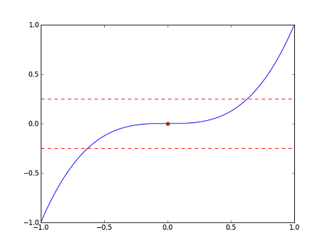
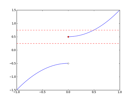
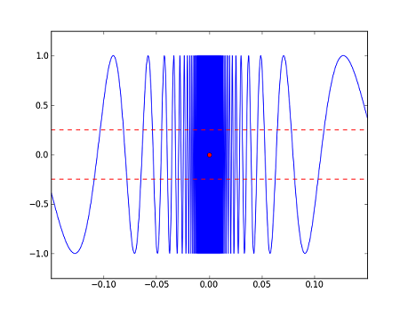
Let's consider the the following three functions along with their graphs (in blue). The red dots in each correspond to $ x=0 $, e.g. for $ f $, the red dot is the point $ (0,f(0))=(0,0) $. Ignore the red dashed lines for now; we will explain them later.
- $ \displaystyle f(x)=x^3 $
- $ g(x)=\begin{cases}-x^2-\frac{1}{2} &\text{if}~x<0\\ x^2+\frac{1}{2} &\text{if}~x\geq 0\end{cases} $
- $ h(x)=\begin{cases} \sin\left(\frac{1}{x}\right) &\text{if}~x\neq 0\\ 0 &\text{if}~x=0\end{cases} $
We can see from the graphs that $ f $ is "continuous" at $ 0 $, and that $ g $ and $ h $ are "discontinuous" at 0. But, what exactly do we mean? Intuitively, $ f $ seems to be continuous at $ 0 $ because $ f(x) $ is close to $ f(0) $ whenever $ x $ is close to $ 0 $. On the other hand, $ g $ appears to be discontinuous at $ 0 $ because there are points $ x $ which are close to $ 0 $ but such that $ g(x) $ is far away from $ g(0) $. The same observation applies to $ h $.
Let's make these observations more precise. First, we will try to estimate $ f(0) $ with error at most $ 0.25 $, say. In the graph of $ f $, we have marked off a band of width $ 0.5 $ about $ f(0) $. So, any point in the band will provide a good approximation here. As a first try, we might think that if $ x $ is close enough to $ 0 $, then $ f(x) $ will be a good estimate of $ f(0) $. Indeed, we see from the graph that for any $ x $ in the interval $ (-\sqrt[3]{0.25},\sqrt[3]{0.25}) $, $ f(x) $ lies in the band (or if we wish to be more pedantic, we would say that $ (x,f(x)) $ lies in the band). So, "close enough to $ 0 $" here means in the interval $ (-\sqrt[3]{0.25},\sqrt[3]{0.25}) $; note that any point which is close enough to $ 0 $ provides a good approximation of $ f(0) $.
There is nothing special about our error bound $ 0.25 $. Choose a positive number $ \varepsilon $, and suppose we would like to estimate $ f(0) $ with error at most $ \varepsilon $. Then, as above, we can find some interval $ \displaystyle(-\delta,\delta) $ about $ 0 $ (if you like to be concrete, any $ \displaystyle\delta $ such that $ 0<\delta<\sqrt[3]{varepsilon} $ will do) such that $ f(x) $ is a good estimate for $ f(0) $ for any $ x $ in $ \displaystyle(-\delta,\delta) $. In other words, for any $ x $ which is close enough to $ 0 $, $ f(x) $ will be no more than $ \varepsilon $ away from $ f(0) $.
Can we do the same for $ g $? That is, if $ x $ is close enough to $ 0 $, then will $ g(x) $ be a good estimate of $ g(0) $? Well, we see from the graph that $ g(0.25) $ provides a good approximation to $ g(0) $. But if $ 0.25 $ is close enough to $ 0 $, then certainly $ -0.25 $ should be too; however, the graph shows that $ g(-0.25) $ is not a good estimate of $ g(0) $. In fact, for any $ x>0 $, $ g(-x) $ will never be a good approximation for $ g(0) $, even though $ x $ and $ -x $ are the same distance from $ 0 $.
In contrast to $ f $, we see that for any interval $ \displaystyle(-\delta,\delta) $ about $ 0 $, we can always find an $ x $ in $ \displaystyle(-\delta,\delta) $ such that $ g(x) $ is more than $ 0.25 $ away from $ g(0) $.
We see that the same is true for $ h $. Whenever we find an $ x_1 $ such that $ h(x_1) $ lies in the band, we can always find a point $ x_2 $ such that 1) $ x_2 $ is just as close or closer to $ 0 $ and 2) $ h(x_2) $ lies outside the band. So, it is not true that if $ x $ is close enough to $ 0 $, then $ h(x) $ will be a good estimate for $ h(0) $.
Let's summarize what we have found. For $ f $, we saw that for each $ \varepsilon>0 $, there is an interval $ \displaystyle(-\delta,\delta) $ about $ 0 $ (note that $ \displaystyle\delta $ depends on $ \varepsilon $) such that $ f(x) $ is in $ (f(0)-\varepsilon,f(0)+\varepsilon) $ for every $ x $ in $ \displaystyle(-\delta,\delta) $.
TOPIC 3
Lorem Ipsum [1] is simply dummy text of the printing and typesetting industry. Lorem Ipsum has been the industry's standard dummy text ever since the 1500s, when an unknown printer took a galley of type and scrambled it to make a type specimen book. It has survived not only five centuries, but also the leap into electronic typesetting, remaining essentially unchanged. It was popularised in the 1960s with the release of Letraset sheets containing Lorem Ipsum passages, and more recently with desktop publishing software like Aldus PageMaker including versions of Lorem Ipsum.
TOPIC 2
Lorem Ipsum [1] is simply dummy text of the printing and typesetting industry. Lorem Ipsum has been the industry's standard dummy text ever since the 1500s, when an unknown printer took a galley of type and scrambled it to make a type specimen book. It has survived not only five centuries, but also the leap into electronic typesetting, remaining essentially unchanged. It was popularised in the 1960s with the release of Letraset sheets containing Lorem Ipsum passages, and more recently with desktop publishing software like Aldus PageMaker including versions of Lorem Ipsum.
REFERENCES
[1] "Loream Ipsum" <http://www.lipsum.com/>.
Questions and comments
If you have any questions, comments, etc. please, please please post them below:
- Comment / question 1
- Comment / question 2
The Spring 2014 Math Squad was supported by an anonymous gift to Project Rhea. If you enjoyed reading these tutorials, please help Rhea "help students learn" with a donation to this project. Your contribution is greatly appreciated.


