| Line 132: | Line 132: | ||
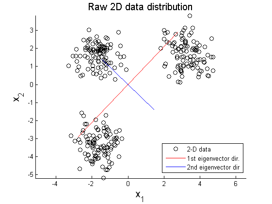
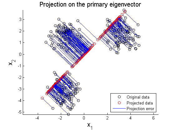
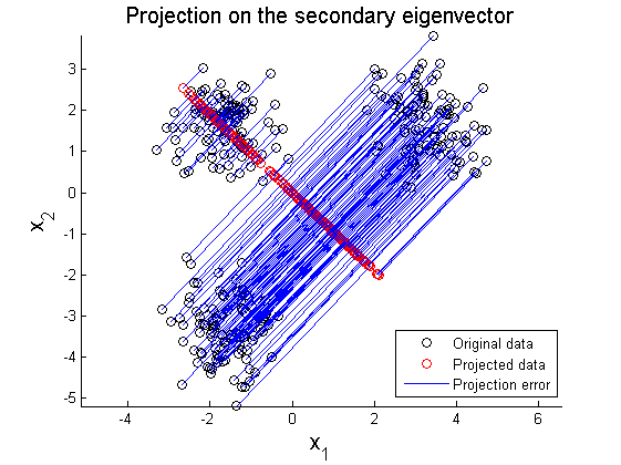
The second example is PCA on multi-Gaussian data distribution. Figure 11 depicts the original data distribution, and PCA results using the principal directions are given in Figure 12 and 13. | The second example is PCA on multi-Gaussian data distribution. Figure 11 depicts the original data distribution, and PCA results using the principal directions are given in Figure 12 and 13. | ||
| − | These two examples show limitations of PCA in dimension reduction. When a given data set is not linearly distributed but might be arranged along with non-orthogonal axes or well described by a geometric parameter, PCA could fail to represent and recover original data from projected variables. For example, by only looking at data distribution projected on the principal direction in Figure 9-10 and 12-13, it is almost impossible to find | + | These two examples show limitations of PCA in dimension reduction. When a given data set is not linearly distributed but might be arranged along with non-orthogonal axes or well described by a geometric parameter, PCA could fail to represent and recover original data from projected variables. For example, by only looking at data distribution projected on the principal direction in Figure 9-10 and 12-13, it is almost impossible to find corresponding original data set. To resolve these issues, in literature, kernel PCA or statistically independent component analysis (ICA) are employed where PCA fails. |
<center>[[Image:ex_3_circular_raw.png]]</center> | <center>[[Image:ex_3_circular_raw.png]]</center> | ||
Revision as of 10:41, 30 April 2014
Basics and Examples of Principal Component Analysis (PCA)
A slecture by Sujin Jang
Partly based on the ECE662 Spring 2014 lecture material of Prof. Mireille Boutin.
Contents
Introduction
Principal Component Analysis (PCA) is one of famous techniqeus for dimension reduction, feature extraction, and data visualization. In general, PCA is defined by a transformation of a high dimensional vector space into a low dimensional space. Let's consider visualization of 10-dim data. It is barely possible to effectively show the shape of such high dimensional data distribution. PCA provides an efficient way to reduce the dimensionalty (i.e., from 10 to 2), so it is much easier to visualize the shape of data distribution. PCA is also useful in the modeling of robust classifier where considerably small number of high dimensional training data is provided. By reducing the dimensions of learning data sets, PCA provides an effective and efficient method for data description and classification.
This lecture is designed to provide a mathematical background of PCA and its applications. First, fundamentals of linear algebra is introduced that will be used in PCA. Technical procedure of PCA will be provided to aid understanding of practical implementation of PCA. Based on the procedure, several examples of PCA will be given in dimension reduction.
Eigenvectors, Eigenvalues, and Singular Vector Decompositoin
For the implementation of PCA, it is important to understand some important concepts in linear algebra. In this lecture, we will briefly discuss eigenvectors and eigenvalues of a matrix. Also singular vector decomposition (SVD) will be examined in the extraction of principal components. More details and examples are directed to [2].
Eigenvectors and Eigenvalues
Let define a n-by-n matrix A and a non-zero vector $ \vec{x}\in\mathbb{R}^{n} $. If there exists a scalar value λ which satisfies the vector equation
we define λ as an eigenvalue of the matrix A, and the corresponding non-zero vector $ \vec{x} $ is called an eigenvector of the matrix A. To determine eigenvalues and eigenvectors a characteristic equation
is used. Here is an example of determining eigenvectors and eigenvalues where the matrix A is given by
Then the characteristic equation is given by
By solving the quadratic equation for λ, we will have two eigenvalues λ1 = − 1 and λ2 = − 6. By substituting λ's into the vector equation, we can obtain corresponding eigenvectors;
Singular Vector Decomposition (SVD)
In the implementation of PCA, singular vector decomposition (SVD) is used to extract principal components (eiegenvectors) from a given data set. Given a n-by-m matrix A, a singular vector decomposition of A is expressed as:
where $ U\in\mathbb{R}^{n\times n},\;\Sigma\in\mathbb{R}^{n\times m},\; V\in\mathbb{R}^{m\times m} $. The matrix U and V are orthogonal matrices, and consist of left and right singular vectors respectively. The matrix Σ is diagonal and consists of non-negative singular values σi. The singular values are placed in Σ in descending order such as
Technical Procedure of PCA
In this section, a brief procedural description of PCA is provided. More detailed theoretical description is directed to [3]. Assume that we are given by a m-by-n data matrix X consists of n number of m-dim vectors $ \vec{x}_{i}\in\mathbb{R}^{m} $.
Step 1: Compute mean and covariance of data matrix
The covariance matrix of X is called $ S\in\mathbb{R}^{m\times m} $ and defined by
where $ \bar{x}\in\mathbb{R}^{m} $ is the mean of each row in X and defined by
Step 2: SVD
Singular vector decomposition of S is implemented to extract principal components and directions:
where $ U\in\mathbb{R}^{n\times n},\;\Sigma\in\mathbb{R}^{n\times m},\; V\in\mathbb{R}^{m\times m} $. In the implementation, we use the matrix $ V=\left[u_{1}u_{2}\cdots u_{m}\right] $ where a vector $ u_{i}\in\mathbb{R}^{m} $ represents a principal component direction.
Step 3: Projection
The data matrix X can be projected into a new matrix $ Y\in\mathbb{R}^{k\times m} $ by multiplying a matrix PT
where $ P=\left[\begin{matrix}u_{1}u_{2}\cdots u_{k}\end{matrix}\right],\; k\leq m $. Proper number of principal components k should be selected in prior to perform projection of data matrix.
Examples
1. 2D data analysis
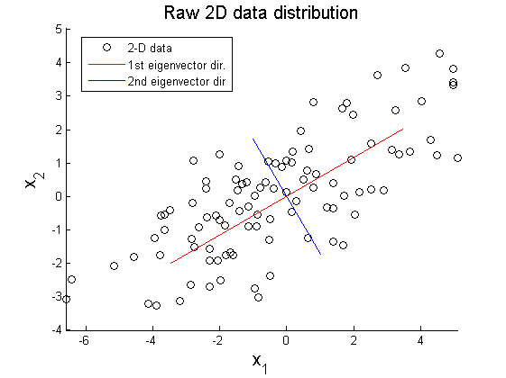
In this example, PCA is implemented to project one hundred of 2-D data $ X\in\mathbb{R}^{2\times100} $ on 1-D space. Figure 1 shows elliptical distribution of X with principal component directions $ \vec{u}_{1} $ and $ \vec{u}_{2} $. The principal directions are extracted from covariance matrix of original data set using SVD method:
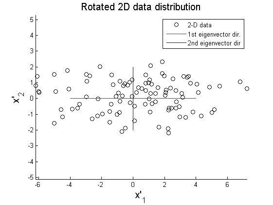
As shown in Figure 2, the data matrix X can be rotated to align principal axes with x and y axis:
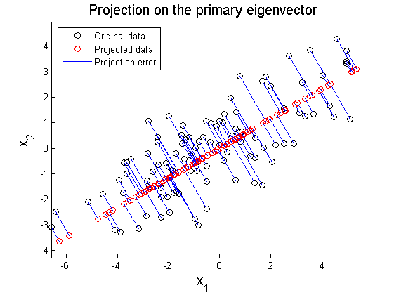
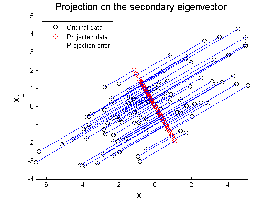
where X' represents rotated data matrix. In Figure 3 and 4, the matrix X is projected on the primary and secondary principal direction. Euclidean distances between original and projected 2D points are computed and summed up to quantitatively show reliability in data representation. Errors for each principal axis projection are 97.9172 (primary axis) and 223.0955 (secondary axis). As a result of PCA, it is observed that selection of proper eigenvector is important for the effective representation of higher dimensional data with lower dimensions while the loss of information is minimized.
2. Image compression
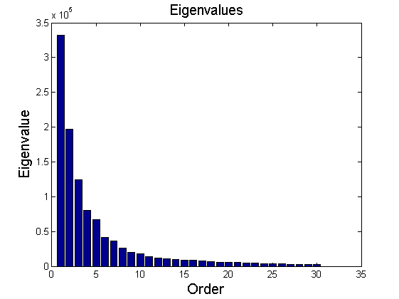
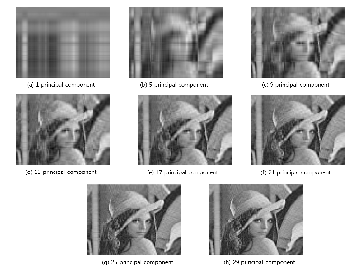
In this example, PCA is applied in the compression of 512-by-512 grey-scale image (Figure 5). The image is represented by a matrix $ X\in\mathbb{R}^{512\times512} $. According to the procedure described in Technical procedure section, principal component directions $ V\in\mathbb{R}^{512\times512} $ is extracted from covariance of the matrix X. Detailed information on implementation is referred to [4]. Figure 6 depicts the first 30 eigenvalues. By only looking at the eigenvalues, it is hard to judge how many principal components are required to effectively represent the original image without loss of generality. As given in Figure 7-(b), even though the first five principal components show relatively large eigenvalues (Figure 6), the projected image does not provide clear correspondence to the original image. Figure 7 shows projection of the original image on new image space defined by different number of principal components. As the number of principal components increases, the projected image becomes visually close to the original image.

3. Nonlinear multimodal data distribution
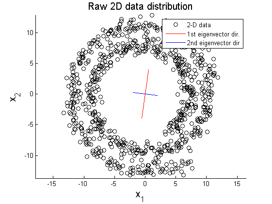
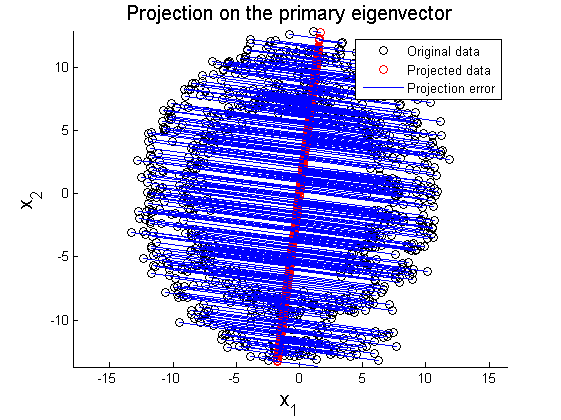
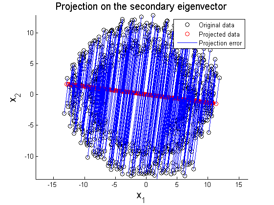
In this section, two examplar cases where PCA fails in data representation are introduced. In the first example, 2D data of circular pattern is analyzed using PCA. Figure 8 shows the original circualr 2D data, and Figure 9 and 10 represent projection of the original data on the primary and secondary principal direction. The second example is PCA on multi-Gaussian data distribution. Figure 11 depicts the original data distribution, and PCA results using the principal directions are given in Figure 12 and 13.
These two examples show limitations of PCA in dimension reduction. When a given data set is not linearly distributed but might be arranged along with non-orthogonal axes or well described by a geometric parameter, PCA could fail to represent and recover original data from projected variables. For example, by only looking at data distribution projected on the principal direction in Figure 9-10 and 12-13, it is almost impossible to find corresponding original data set. To resolve these issues, in literature, kernel PCA or statistically independent component analysis (ICA) are employed where PCA fails.
Discussion
In the lecture, we have covered fundamental background in linear algebra for PCA implementation, practical procedure of PCA, and its application with some examples. As observed in the examples, PCA is a simple but effective method to reduce dimensions of linearly distributed data. Image data compression using PCA shows an efficient way to store huge imagery data with reduced dimensions and without loss of generality. However, in general situ, a-prior knowledge of the data shape is strongly required to attain satisfying PCA result. If the given data set is nonlinear or multimodal distribution, PCA fails to provide meaningful data reduction. To incorporate the prior knowledge of data to PCA, researchers have proposed dimension reduction techniques as extensions of PCA such as kernel PCA, multilinear PCA, and independent component analysis (ICA).
References
- Mireille Boutin, "ECE662: Statistical Pattern Recognition and Decision Making Processes," Purdue University, Spring 2014.
- Erwin Kreyszig, "Advanced Engineering Mathematics (10th edition)", John Wiley & Sons, Inc.
- Christoper M. Bishop, "Pattern recognition and machine learning". 2006, Springer.
- Mark Richardson, "Principal Component Analysis", lecture note on May 2009, (http://people.maths.ox.ac.uk/richardsonm/SignalProcPCA.pdf)
Matlab Code
All the implemented Matlab codes are attached below
Questions and comments
If you have any questions, comments, etc. please post them on this page.

