| (10 intermediate revisions by one other user not shown) | |||
| Line 1: | Line 1: | ||
[[Category:ECE637]] | [[Category:ECE637]] | ||
[[Category:Slecture]] [[Category:ECE438Fall2014Boutin]] [[Category:ECE]] [[Category:ECE438]] [[Category:Signal_processing]] | [[Category:Slecture]] [[Category:ECE438Fall2014Boutin]] [[Category:ECE]] [[Category:ECE438]] [[Category:Signal_processing]] | ||
| + | [[Category:honors project]] | ||
| − | |||
<center><font size="5"></font> | <center><font size="5"></font> | ||
<font size="5">Magnetic Resonance Imaging (MRI)</font> | <font size="5">Magnetic Resonance Imaging (MRI)</font> | ||
| Line 13: | Line 13: | ||
=Introduction= | =Introduction= | ||
| − | Magnetic Resonance Imaging (MRI) is a different mode of imaging from the previously discussed ones. It is characterized by using changing magnetic fields and RF waves to selectively resonate areas of interest for imaging. MRI does not use ionizing radiation like CT does, and it is very flexible and adaptable. It can be reprogrammed to fit specific needs. It is also very high in resolution with normal scans having a resolution on the order of millimeters. Theoretically the only bound on the resolution is | + | Magnetic Resonance Imaging (MRI) is a different mode of imaging from the previously discussed ones. It is characterized by using changing magnetic fields and RF waves to selectively resonate areas of interest for imaging. MRI does not use ionizing radiation like CT does, and it is very flexible and adaptable. It can be reprogrammed to fit specific needs. It is also very high in resolution with normal scans having a resolution on the order of millimeters. Theoretically the only bound on the resolution is how long you want to run the scan. This quality has its trade-offs. MRI is very expensive and the length of the scan is long. A big superconducting magnet, which is very expensive, is needed. Despite these drawbacks, MRI has many different uses. It can be used for conventional anatomical scans, as a functional imaging modality (oxygen activity levels in the brain), and as other modalities. |
[[Image: MRI_scanner.jpg|400px|thumb|left|Fig 1: An MRI Scanner]] | [[Image: MRI_scanner.jpg|400px|thumb|left|Fig 1: An MRI Scanner]] | ||
| Line 62: | Line 62: | ||
The width and location of the desired slice can be modified by the characteristics of the pulse emitted by the RF antenna. In order to send the pulse, it needs to be modulated onto a carrier wave. This modulation causes the frequency response of the RF signal to be a shifted rect. The shift is determined by the carrier wave, and the width of the slice corresponds the the width of the rect. | The width and location of the desired slice can be modified by the characteristics of the pulse emitted by the RF antenna. In order to send the pulse, it needs to be modulated onto a carrier wave. This modulation causes the frequency response of the RF signal to be a shifted rect. The shift is determined by the carrier wave, and the width of the slice corresponds the the width of the rect. | ||
| − | There are 2 design parameters: | + | There are 2 design parameters:<br /> |
<math>z_c:</math>= slice center, controlled by the carrier frequency<br /> | <math>z_c:</math>= slice center, controlled by the carrier frequency<br /> | ||
| − | <math>\ | + | <math>\Delta z:</math>= slice thickness, controlled by the width of the sinc pulse<br /> |
To focus on the slice centered at <math>z_c</math>, the pulse frequency is given by <br/> | To focus on the slice centered at <math>z_c</math>, the pulse frequency is given by <br/> | ||
| Line 89: | Line 89: | ||
<math>r(x,y,t) = f(x,y)e^{j\phi (t)} \ </math><br /> | <math>r(x,y,t) = f(x,y)e^{j\phi (t)} \ </math><br /> | ||
<math>f(x,y)</math> is the quantity of interest that is dependent on the properties of the material in the voxel and a weighting (T1,T2 or T2*)<br /> | <math>f(x,y)</math> is the quantity of interest that is dependent on the properties of the material in the voxel and a weighting (T1,T2 or T2*)<br /> | ||
| − | <math>\phi (t)</math> is the phase of the received signal. This term can be modulated using <math>G_x</math> and <math>G_y</math>. Also | + | <math>\phi (t)</math> is the phase of the received signal. This term can be modulated using <math>G_x</math> and <math>G_y</math>. Also without loss of generality, we assume that <math>\phi (0) = 0</math>. Any complex constant is absorbed into <math>f(x,y)</math>. |
| + | |||
| + | For a signal with phase <math>\phi (t)</math>, the instantaneous frequency <math>v(t)</math> is the time derivative of the phase.<br /> | ||
| + | <math>f(t) = \frac{d\phi (t)}{dt}</math><br /> | ||
| + | <math>\Rightarrow \phi (t) = \int_{-\infty}^{t} f(\tau)d\tau</math><br /> | ||
| + | From here we can relate the oscillation frequency (<math>\omega = LM</math>) to the instantaneous frequency. <br /> | ||
| + | <math>\begin{align} | ||
| + | \frac{d\phi(t)}{dt} &= LM(x,y,t) \\ | ||
| + | \Rightarrow \phi(t) &= \int_0^t LM(x,y,\tau)d\tau \\ | ||
| + | &= \int_0^t (LM_0 + xLG_x(\tau) + yLG_y(\tau))d\tau \\ | ||
| + | &= \omega_0t + xk_x(t) +yk_y(t) | ||
| + | \end{align}</math> <br /> | ||
| + | Where<br /> | ||
| + | <math>\begin{align} | ||
| + | w_0 &= LM_o \\ | ||
| + | k_x (t) &= \int_0^t LG_x (\tau)d\tau \\ | ||
| + | k_y (t) &= \int_0^t LG_y (\tau)d\tau | ||
| + | \end{align}</math> | ||
| + | <br /> | ||
| + | Plugging this back into formula for the RF signal emitted from a single voxel<br /> | ||
| + | <math>\begin{align} | ||
| + | r(x,y,t) &= f(x,y)e^{j\phi(t)} \\ | ||
| + | &= f(x,y)e^{j(\omega_0t + xk_x(t) + yk_y(t))} \\ | ||
| + | &= f(x,y)e^{j\omega_0t}e^{j(xk_x(t) + yk_y(t))} | ||
| + | \end{align}</math><br /> | ||
| + | |||
| + | This result can be broken down into the carrier sinusoid <math>e^{j\omega_0 t}</math> and the phase modulation <math>e^{j(xk_x(t) + yk_y(t))}</math> added by the gradients <math>G_x</math> and <math>G_y</math>. To extract actual value of interest <math>f(x,y)</math>, the emitted RF signal must be demodulated. | ||
---- | ---- | ||
=Scaling Signal Analysis to a Slice= | =Scaling Signal Analysis to a Slice= | ||
| − | =K-Space= | + | The RF signal from the complete slice is given by combining the contributions from all the voxels in that slice, so we integrate to get <br/> |
| + | <math>\begin{align} | ||
| + | R(t) &= \int_{\mathbb{R}}\int_{\mathbb{R}}r(x,y,t)dxdy \\ | ||
| + | &= \int_{\mathbb{R}}\int_{\mathbb{R}} f(x,y)e^{j\omega_0t}e^{j(xk_x(t) + yk_y(t))}dxdy \\ | ||
| + | &= e^{j\omega_0t}\int_{\mathbb{R}}\int_{\mathbb{R}} f(x,y)e^{j(xk_x(t) + yk_y(t))}dxdy \\ | ||
| + | &= e^{j\omega_0t}F(-k_x(t),-k_y(t)) \ \text{, by comparison with CSFT} \\ | ||
| + | R(t)e^{-j\omega_0 t} &= F(-k_x(t),-k_y(t)) | ||
| + | \end{align}</math> | ||
| + | |||
| + | where <math>F(u,v) </math> is the CSFT of <math>f(x,y)</math>, <math>u = -k_x(t)</math> and <math>v = -k_y(t)</math>. Now we have that the demodulated received signal is the CSFT of the object evaluated at specific phases. Essentially a MRI scan is the Fourier Transform of a person. | ||
| + | ---- | ||
| + | =K-Space Interpretation= | ||
| + | |||
| + | The K in K-space refers to the wave number of the signal. The RF signal from the complete slice is given by <br /> | ||
| + | <math>F(-k_x(t),-k_y(t)) = R(t)e^{-j\omega_0 t}</math> <br /> | ||
| + | By scanning through spatial frequencies by varying <math>k_x(t)</math> and <math>k_y(t)</math>, the image can be reconstructed by performing the inverse CSFT. | ||
| + | |||
| + | By relating the gradient coil voltage and the K-space, we can choose the speed with which we scan through the slice. Since the gradients are coils, it can be observed that<br /> | ||
| + | <math>\begin{matrix} | ||
| + | L_x\frac{di(t)}{dt} = v_x(t) & G_x(t) = M_xi(t) \\ | ||
| + | L_y\frac{di(t)}{dt} = v_y(t) & G_y(t) = M_yi(t) | ||
| + | \end{matrix}</math><br /> | ||
| + | <math>L_x</math> and <math>L_y</math> are the coil inductances while <math>v_x(t)</math> and <math>v_y(t)</math> are the voltages across the coil. Using these relationships, we get<br /> | ||
| + | <math>\begin{align} | ||
| + | k_x(t) &= \int_0^t LG_x(\tau)d\tau \\ | ||
| + | &= \int_0^t LM_xi(\tau)d\tau \\ | ||
| + | &= LM_x \int_0^t i(\tau)d\tau \text{, note that } i(t)&= \int_0^{\tau} \frac{v_x(\tau)}{L_x}d\tau \\ | ||
| + | &= \frac{LM_x}{L_x}\int_0^t\int_0^{\tau}v_x(s)dsd\tau \\ | ||
| + | \Rightarrow k_y(t) &= \frac{LM_y}{L_y}\int_0^t\int_0^{\tau}v_y(s)dsd\tau | ||
| + | \end{align}</math><br /> | ||
| + | |||
| + | An analogy can be made between the acceleration of a particle being the second derivative and the voltage of the coil being the acceleration through k-space. Because the voltage is the independent variable in this case, it can be changed to scan through various magnetic gradients focusing on specific voxels across a slice. | ||
| + | ---- | ||
=Echo Planar Imaging (EPI) Scan Pattern= | =Echo Planar Imaging (EPI) Scan Pattern= | ||
| − | + | The EPI scan pattern in Figure 6 shows a commonly used path to scan through K-space. As mentioned above, the movement through K-space can be controlled by the coil voltages, so Figure 7 shows the pulses in coil voltage and the resulting the change in the magnetic gradient speed that is associated with the EPI scan pattern in Figure 6. The scanning pattern creates the CSFT of which an inverse can be taken to construct the original slice. Repeating the process for all slices of interest will build a 3D model of the patient. <br /> | |
| − | + | ||
| + | [[Image:MRI_EPI.jpg|400px|thumb|left|Fig 6: A Common EPI Path]] | ||
| + | [[Image:MRI_EPI_control.jpg|400px|thumb|left|Fig 7: Coil Voltage Pulses and Resulting Velocity Changes]] | ||
| + | ---- | ||
References:<br /> | References:<br /> | ||
[1] C. A. Bouman. ECE 637. Class Lecture. Digital Image Processing I. Faculty of Electrical Engineering, Purdue University. Spring 2013. <br /> | [1] C. A. Bouman. ECE 637. Class Lecture. Digital Image Processing I. Faculty of Electrical Engineering, Purdue University. Spring 2013. <br /> | ||
| − | + | ---- | |
| + | =Questions and Comments= | ||
| + | Please post your questions and comments on the [[ECE438HonorsContractDiscuss|discussion page.]] | ||
| + | ---- | ||
[[ HonorsContractECE438Fall14|Back to Honors Contract Main Page]] | [[ HonorsContractECE438Fall14|Back to Honors Contract Main Page]] | ||
Latest revision as of 19:26, 9 February 2015
Magnetic Resonance Imaging (MRI)
A slecture by ECE student Sahil Sanghani
Partly based on the ECE 637 material of Professor Bouman.
Contents
- 1 Introduction
- 2 Magnetic Resonance
- 3 MRI Hardware
- 4 Magnetic Field Gradients
- 5 MRI Slice Selection
- 6 Slice Selection Pulse Design
- 7 Image the Selected Slice
- 8 Signal Analysis on a Single Voxel
- 9 Scaling Signal Analysis to a Slice
- 10 K-Space Interpretation
- 11 Echo Planar Imaging (EPI) Scan Pattern
- 12 Questions and Comments
Introduction
Magnetic Resonance Imaging (MRI) is a different mode of imaging from the previously discussed ones. It is characterized by using changing magnetic fields and RF waves to selectively resonate areas of interest for imaging. MRI does not use ionizing radiation like CT does, and it is very flexible and adaptable. It can be reprogrammed to fit specific needs. It is also very high in resolution with normal scans having a resolution on the order of millimeters. Theoretically the only bound on the resolution is how long you want to run the scan. This quality has its trade-offs. MRI is very expensive and the length of the scan is long. A big superconducting magnet, which is very expensive, is needed. Despite these drawbacks, MRI has many different uses. It can be used for conventional anatomical scans, as a functional imaging modality (oxygen activity levels in the brain), and as other modalities.
Magnetic Resonance
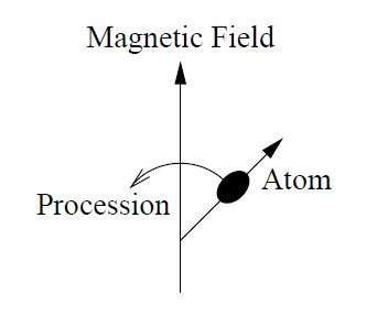
Atoms that have a magnetic dipole process around the magnetic field's axis, not unlike how a top takes a wider rotation as slows down. Figure 2 shows how these atoms process.
Different atoms have different procession frequencies, which is called the Lamor Frequency, based on intrinsic qualities and the surrounding magnetic field. Hydrogen is the typical atom of focus in conventional MRI scanners due to its ubiquity in the water contained in the soft tissue of the body. At a magnetic field strength of 1.5T, the Lamor frequency for H is 63 MHz.
Let
$ M: $= magnitude of the magnetic field
$ \omega_0: $= the frequency of procession (Lamor frequency)
$ L: $= Lamor constant, which is an intrinsic atomic quality
The Lamor frequency is defined as
$ \omega_0 = LM \ $
The procession can resonate with an RF signal targeted at the atom if the RF signal is at the center frequency of procession. Once the RF signal is removed, the atom will radiate RF energy until the energy is lost. The sensitivity of procession to magnetic field is used to selectively choose slices for analysis, and the RF energy emission is used to create pinpoint specific nuclei of interest. This data makes up the projections used in reconstruction.
MRI Hardware
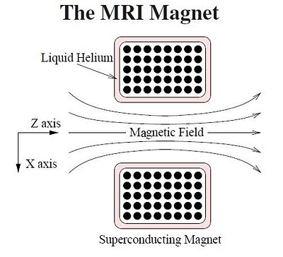
Clinically high strength magnetic fields are used for imaging because ensure good resolution. Also, the radius of the bore where the patient enters the scanner is relatively large, so stronger fields are needed to compensate. In order to generate these large magnetic fields, superconducting magnets are used.
Superconducting magnets are metals whose resistance is 0$ \Omega $ when they are cooled to below a threshold temperature. Liquid helium is used to achieve these low temperatures, which are around a few degrees Kelvin. Because Helium is the lightest noble gas, it is the lightest and one of the faster moving inert substances. It is so energetic that it only changes phase at extremely low temperatures. At normal pressures, solid helium doesn't even exist because it is impossible for the atoms to be fixed in an ordered structure.
Once electric current is injected into the superconducting magnet by a generator, it continuously flows. Because there is no resistance, the amount of current doesn't decrease and just keeps flowing even when the generator is disconnected. The orientation of all the elements in the magnetic field generation is shown in Figure 3.
Over time some of the liquid helium will boil off, and leave the superconducting magnet exposed. This is an event known as "quenching." As the superconducting magnet is left exposed, it warms up and gains a little resistance. This little resistance starts a vicious cycle of heat dissipation and further helium boiled off. This exponential increase in helium converting to gas can be destructive, so the magnets have to be designed accordingly.
Magnetic Field Gradients
For our purposes, we will assume that the magnetic field created by the superconducting magnet is a scalar ($ M_o $) with a position independent yet adjustable magnitude as opposed to a vector. This is assumption is made because the field within the bore should be flowing in a fixed direction.
On top of having the superconducting magnet, there are magnetic gradient coils that can slightly alter the field withing the bore. The gradient coils are designed so that the magnetic field changes linearly with position, and they are controlled through amplifiers. These gradients go along each axis, and are named $ G_x $, $ G_y $ and $ G_z $. Thus the magnetic field magnitude at the location $ (x,y,z) $ can be expressed as
$ M(x,y,z) = M_o + xG_x + yG_y + zG_z \ $
For the time changing gradients the expression can be adapted as follows
$ M(x,y,z,t) = M_o + xG_x(t) + yG_y(t) + zG_z(t) \ $
The current through each of the three coils, one for each axis, enable a gradient to be created/adjusted along each axis.
MRI Slice Selection
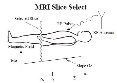
For this explanation, assume that the $ G_x=G_y=0 $. We will have a positive gradient from $ G_z $ as shown in Figure 4.
Now if an RF pulse at 63MHz is sent to the body, protons whose resonant frequency matches the RF frequency will resonate. Because there is a magnetic gradient, the atoms at different values of $ z $ have different resonant frequencies. Changing the frequency of the RF pulse would allow the targeting of specific values of $ z $. Because all the H atoms at a specific value of $ z $ will have the same magnetic field, they would all be targeted by a specific RF frequency. This group makes up the "slice" of the person being selectively excited.
Essentially the resonance frequency of the H atoms is given by
$ \omega = L(M_o + zG_z) \ $
Slice Selection Pulse Design
The width and location of the desired slice can be modified by the characteristics of the pulse emitted by the RF antenna. In order to send the pulse, it needs to be modulated onto a carrier wave. This modulation causes the frequency response of the RF signal to be a shifted rect. The shift is determined by the carrier wave, and the width of the slice corresponds the the width of the rect.
There are 2 design parameters:
$ z_c: $= slice center, controlled by the carrier frequency
$ \Delta z: $= slice thickness, controlled by the width of the sinc pulse
To focus on the slice centered at $ z_c $, the pulse frequency is given by
$ f_c = \frac{LM_o}{2\pi}+\frac{z_cLG_z}{2\pi} = f_0 + \frac{z_cLG_z}{2\pi} $
The pulse bandwidth can be calculated from the slice thickness $ \Delta z $
$ BW = \frac{\Delta z LG_z}{2\pi} $
Using the parameters $ f_c $ and $ BW $, the pulse is given by
$ p(t) = e^{j2\pi f_ct}sinc(tBW) $
and its CTFT is given by
$ P(f) = rect(\frac{f-f_c}{BW}) $
Image the Selected Slice
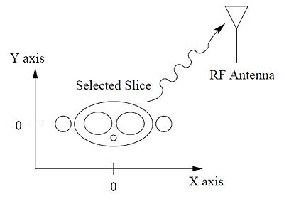
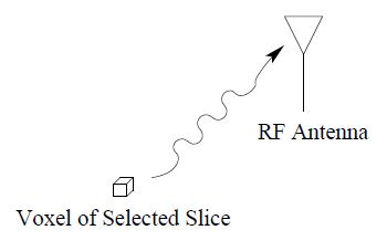
Previously we saw how to target a specific slice, but just recording the volume of RF emission from a total slice isn't useful for getting precise reconstruction. The strategy is to vary magnetic gradients $ G_x $ and $ G_y $. This varying will create voxels with individual RF emission amounts that can be compiled into an overall density map of the slice.
Signal Analysis on a Single Voxel
First the signal will be analyzed for a single voxel, then it will be scaled up to calculating every voxel in a slice. Because the calculation is being performed in a single slice, $ z $ is considered a constant.
The RF signal from a single voxel has the form
$ r(x,y,t) = f(x,y)e^{j\phi (t)} \ $
$ f(x,y) $ is the quantity of interest that is dependent on the properties of the material in the voxel and a weighting (T1,T2 or T2*)
$ \phi (t) $ is the phase of the received signal. This term can be modulated using $ G_x $ and $ G_y $. Also without loss of generality, we assume that $ \phi (0) = 0 $. Any complex constant is absorbed into $ f(x,y) $.
For a signal with phase $ \phi (t) $, the instantaneous frequency $ v(t) $ is the time derivative of the phase.
$ f(t) = \frac{d\phi (t)}{dt} $
$ \Rightarrow \phi (t) = \int_{-\infty}^{t} f(\tau)d\tau $
From here we can relate the oscillation frequency ($ \omega = LM $) to the instantaneous frequency.
$ \begin{align} \frac{d\phi(t)}{dt} &= LM(x,y,t) \\ \Rightarrow \phi(t) &= \int_0^t LM(x,y,\tau)d\tau \\ &= \int_0^t (LM_0 + xLG_x(\tau) + yLG_y(\tau))d\tau \\ &= \omega_0t + xk_x(t) +yk_y(t) \end{align} $
Where
$ \begin{align} w_0 &= LM_o \\ k_x (t) &= \int_0^t LG_x (\tau)d\tau \\ k_y (t) &= \int_0^t LG_y (\tau)d\tau \end{align} $
Plugging this back into formula for the RF signal emitted from a single voxel
$ \begin{align} r(x,y,t) &= f(x,y)e^{j\phi(t)} \\ &= f(x,y)e^{j(\omega_0t + xk_x(t) + yk_y(t))} \\ &= f(x,y)e^{j\omega_0t}e^{j(xk_x(t) + yk_y(t))} \end{align} $
This result can be broken down into the carrier sinusoid $ e^{j\omega_0 t} $ and the phase modulation $ e^{j(xk_x(t) + yk_y(t))} $ added by the gradients $ G_x $ and $ G_y $. To extract actual value of interest $ f(x,y) $, the emitted RF signal must be demodulated.
Scaling Signal Analysis to a Slice
The RF signal from the complete slice is given by combining the contributions from all the voxels in that slice, so we integrate to get
$ \begin{align} R(t) &= \int_{\mathbb{R}}\int_{\mathbb{R}}r(x,y,t)dxdy \\ &= \int_{\mathbb{R}}\int_{\mathbb{R}} f(x,y)e^{j\omega_0t}e^{j(xk_x(t) + yk_y(t))}dxdy \\ &= e^{j\omega_0t}\int_{\mathbb{R}}\int_{\mathbb{R}} f(x,y)e^{j(xk_x(t) + yk_y(t))}dxdy \\ &= e^{j\omega_0t}F(-k_x(t),-k_y(t)) \ \text{, by comparison with CSFT} \\ R(t)e^{-j\omega_0 t} &= F(-k_x(t),-k_y(t)) \end{align} $
where $ F(u,v) $ is the CSFT of $ f(x,y) $, $ u = -k_x(t) $ and $ v = -k_y(t) $. Now we have that the demodulated received signal is the CSFT of the object evaluated at specific phases. Essentially a MRI scan is the Fourier Transform of a person.
K-Space Interpretation
The K in K-space refers to the wave number of the signal. The RF signal from the complete slice is given by
$ F(-k_x(t),-k_y(t)) = R(t)e^{-j\omega_0 t} $
By scanning through spatial frequencies by varying $ k_x(t) $ and $ k_y(t) $, the image can be reconstructed by performing the inverse CSFT.
By relating the gradient coil voltage and the K-space, we can choose the speed with which we scan through the slice. Since the gradients are coils, it can be observed that
$ \begin{matrix} L_x\frac{di(t)}{dt} = v_x(t) & G_x(t) = M_xi(t) \\ L_y\frac{di(t)}{dt} = v_y(t) & G_y(t) = M_yi(t) \end{matrix} $
$ L_x $ and $ L_y $ are the coil inductances while $ v_x(t) $ and $ v_y(t) $ are the voltages across the coil. Using these relationships, we get
$ \begin{align} k_x(t) &= \int_0^t LG_x(\tau)d\tau \\ &= \int_0^t LM_xi(\tau)d\tau \\ &= LM_x \int_0^t i(\tau)d\tau \text{, note that } i(t)&= \int_0^{\tau} \frac{v_x(\tau)}{L_x}d\tau \\ &= \frac{LM_x}{L_x}\int_0^t\int_0^{\tau}v_x(s)dsd\tau \\ \Rightarrow k_y(t) &= \frac{LM_y}{L_y}\int_0^t\int_0^{\tau}v_y(s)dsd\tau \end{align} $
An analogy can be made between the acceleration of a particle being the second derivative and the voltage of the coil being the acceleration through k-space. Because the voltage is the independent variable in this case, it can be changed to scan through various magnetic gradients focusing on specific voxels across a slice.
Echo Planar Imaging (EPI) Scan Pattern
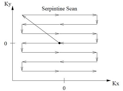
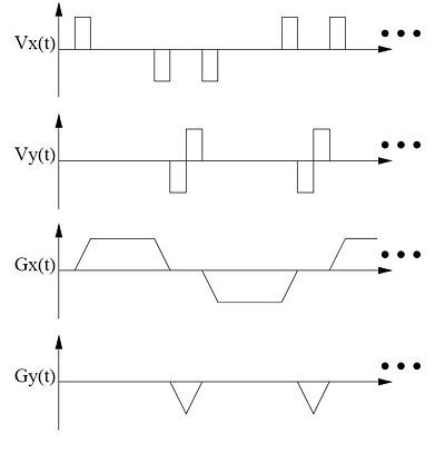
The EPI scan pattern in Figure 6 shows a commonly used path to scan through K-space. As mentioned above, the movement through K-space can be controlled by the coil voltages, so Figure 7 shows the pulses in coil voltage and the resulting the change in the magnetic gradient speed that is associated with the EPI scan pattern in Figure 6. The scanning pattern creates the CSFT of which an inverse can be taken to construct the original slice. Repeating the process for all slices of interest will build a 3D model of the patient.
References:
[1] C. A. Bouman. ECE 637. Class Lecture. Digital Image Processing I. Faculty of Electrical Engineering, Purdue University. Spring 2013.
Questions and Comments
Please post your questions and comments on the discussion page.


