Anonymous7 (Talk | contribs) |
Anonymous7 (Talk | contribs) |
||
| Line 34: | Line 34: | ||
In discrete case, Bayes rule formula is given by, | In discrete case, Bayes rule formula is given by, | ||
| + | <math>P(x|y) = \frac{P(y|x) \cdot P(x)}{P(y)} (5) </math> | ||
| + | |||
| + | <math> f_{X|Y} (x|y) = \frac{ f_{Y|X} (y|x) \times f_{X} (x) } { f_{Y} (y) } (11) </math> | ||
Revision as of 04:42, 1 May 2014
Derivation of Bayes Rule
A slecture by ECE student Anonymous7
Partly based on the ECE662 Spring 2014 lecture material of Prof. Mireille Boutin.
Contents
What will you learn from this slecture?
- Bayes rule statement.
- Derivation of Bayes' rule in discrete and continuous cases.
- An example that illustrates Bayes rule and how it can be used to update or revise the probability.
Introduction
Bayes Rule is an important rule in probability theory that allows to update or revise our theories when new evidence is given. Bayes rule can be used to help us reach decisions and make intuitive and meaningful inferences.
Bayes Rule Statement
In discrete case, Bayes rule formula is given by,
$ P(x|y) = \frac{P(y|x) \cdot P(x)}{P(y)} (5) $
$ f_{X|Y} (x|y) = \frac{ f_{Y|X} (y|x) \times f_{X} (x) } { f_{Y} (y) } (11) $
Derivation of Bayes' Rule
Now, we will consider the derivation of Bayes rule both in discrete and continues cases.
Discrete Random Variables
In discrete case, we have the discrete conditional probability formula,
$ P(x|y)=\frac{P(x \cap y)}{P(y)} (1) $
Now, we can rewrite this equation as
$ P(x \cap y)= P(x|y) \cdot P(y) (2) $
Now, because the intersection is commutative, we can write the P(x \cap y) as,
$ P(x \cap y)= P(y \cap x) (3) $
Now, using the conditional probability definition, we can write equation (3) as
$ P(x|y) \cdot P(y)= P(y|x) \cdot P(x) (4) $
Now, we can write equation 4 as,
$ P(x|y) = \frac{P(y|x) \cdot P(x)}{P(y)} (5) $
Continues Random Variables
Now, we can consider the Bayes' rule when we have continuous random variables. We know that the conditional probability for the continues random variables is,
$ f_{X|Y} (x|y) = \frac{f_{X,Y} (x,y)}{f_{Y} (y)} (6) $
Now, we can write another equation similar to equation 6,
$ f_{Y|X} (y|x) = \frac{f_{Y,X} (y,x)}{f_{X} (x)} (7) $
But because fY,X(y,x) is the same as fX,Y(x,y),i.e., intersection is commutative, we can rewrite equation 7 as follows,
$ f_{Y|X} (y|x) = \frac{f_{X,Y} (x,y)}{f_{X} (x)} (8) $
Now, be rearranging equations 6 and 8, we can write,
$ f_{X,Y} (x,y)= f_{X|Y} (x|y) \times f_{Y} (y) (9) $
$ f_{X,Y} (x,y)= f_{Y|X} (y|x) \times f_{X} (x) (10) $
Now, by equating equations 9 and 10, we get Bayes rule for continues random variables
$ f_{X|Y} (x|y) = \frac{ f_{Y|X} (y|x) \times f_{X} (x) } { f_{Y} (y) } (11) $
Example
Let us suppose that a school has 200 students. 45 students are members of a certain club. At the beginning of the academic year, the school offered a seminar which was attended by 70 students. 25 students, who are members of the club, attended the seminar.
Now, let’s suppose that the probability that a student is a member of the club is $ \textbf{ P}(A) $ and the probability a student is not a member of the club is$ \textbf{ P}(A^c) $. Let suppose $ \textbf{ P}(B) $ is the probability that a student attended the seminar and $ \textbf{ P}(B^c) $ is the probability that a student did not attend the seminar. We can easily see that $ \textbf{ P}(A)=45/200 $ , $ \textbf{ P}(A^c)=155/200 $ , $ \textbf{ P}(B)=70/200 $ , and $ \textbf{ P}(B^c) = 130/200 $
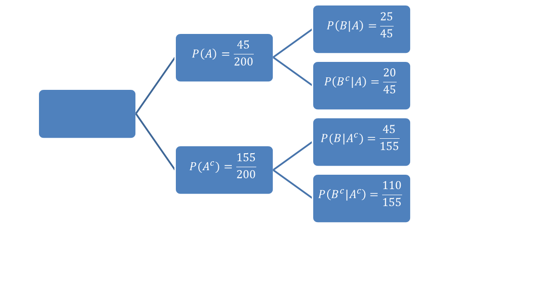
We can find the conditional probabilities as shown in fig.1.
Now, let’s try to answer the following question: What is the probability that a student who attended the seminar is a member of the club? We answer this question easily by using Bayes rule, We know that $ P(A|B) = \frac{P(B|A) \cdot P(A)}{P(B)} $
So, we can calculate $ P(A|B) = \frac{ \frac{25}{45} \cdot \frac{45}{200} } { \frac{70}{200} } = \frac {5}{14} $
Now, Let us try to answer another question: What is the probability that a student who did NOT attend the seminar is a member of the club? Again, we answer this question by using Bayes rule, We know that $ P(A|B^c) = \frac{P(B^c|A) \cdot P(A)}{P(B^c)} $
So, we can calculate $ P(A|B^c) = \frac{ \frac{20}{45} \cdot \frac{45}{200} } { \frac{130}{200} } = \frac {2}{13} $
Now, Let us try to answer another question: What is the probability that a student who attended the seminar is NOT a member of the club? Again, we answer this question by using Bayes rule, We know that $ P(A^c|B) = \frac{P(B|A^c) \cdot P(A^c)}{P(B)} $
So, we can calculate $ P(A^c|B) = \frac{ \frac{45}{155} \cdot \frac{155}{200} } { \frac{70}{200} } = \frac {45}{70} $
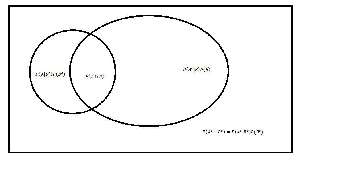
We can see the Venn diagram shown in fig.2.
We can see now that $ \textbf{ P}(A|B) > \textbf{P}(A) $.
Why does the probability change after we know that a student attended the seminar?
When we calculate P(A), we calculate it solely based on our knowledge of the number of students who are members of the club. We don't have any extra information. However, when we calculate the probability after we know a student attended the seminar, the sample space changed from the total number of students to those students who attended the seminar. Therefore, we updated or revised our belief when additional information was given.
References
- ECE662: Statistical Pattern Recognition and Decision Making Processes, Purdue University, Spring 2014.
Questions and comments
If you have any questions, comments, etc. please post them on this page.


