My use for the DFT
In ECE 301 students were introduced to the concept of Fourier Transforms. No matter whom you had been taught by it seemed intimidating and confusing. And irrelevant. They tried to show you where and how it was used but honestly how long did it take for you to finally realize its use? For me two semesters! There were CTFTs, DTFTs and DFTs (and I am sure there are more that I have not been introduced to yet) and they were all a blur of equations that sometimes gave me nightmares. I am not a very mathematical person: I like engineering concepts and ideas but dislike the math behind it because the equations often stop making sense after the fifth Greek letter has been added. So the goal should be to make such math (these transforms rather) and relate them to real life, not just by telling us where it used but by telling us how it is. So I am going to attempt to do that with my limited knowledge of the math that goes one behind the screen.
What is a Fourier Transform?
A Fourier Transform (FT for short) is just an equation that allows us to from the time domain to the frequency domain and the inverse FT performs the reverse. The time domain is just the real time representation of our signal; how the signal varies over time whereas the frequency domain shows us the number of times the main component of a signal repeats per second.
In the time domain you look at the value of something as it changes over time - a series of snapshots, if you will. In the Fourier domain you look at the entire lifetime of the signal all at once - and analyze it in terms of the underlying frequencies that made it up. This means you can no longer see the value at any one time, or the rate at which the signal is changing at any one time. Instead, for each possible frequency, you see the amplitude of the signal at that frequency (such a distribution is called a frequency spectrum).
It is thus a technique that can be used to describe almost anything in the world be it an electric signal or the stock market. Did you know that our brain picks up different frequencies around us and performs a Fourier analysis (really quickly and effectively) on data: for example on different voices, or recognizes differences in high and low notes or just perceives different colors? Scientists haven’t yet found out how all that is done but they know for sure that something of that sort goes on in our highly complex brains.
CTFTs, DTFTs and DFTs
CTFT
$ \mathcal{X}(f) = \int_{-\infty}^{\infty} x(t) e^{-j 2 \pi f t} dt $
A CTFT( continuous time fourier transform) is continuous in both the time and frequency domain. Give example here.
DTFT
$ X(\omega) = \sum_{n=-\infty}^{\infty} x[n] \,e^{-i \omega n}. $
A DTFT (discrete time fourier transform) is performed on signals which are discrete in the time domain but are continuous in the frequency domain.the DTFT requires an input function that is discrete. Such inputs are often created by sampling a continuous function, like a person's voice where the air expelled from the lungs is continuous (signal) and then the vocal tracts take samples of it, periodically to produce a discrete signal. Often the $ x[n]\, $ sequence represents the values (aka samples) of a continuous-time function, $ x(t)\, $, at discrete moments in time: $ t = nT\, $, where $ T\, $ is the sampling interval (in seconds), and $ 1/T = f_s\, $ is the sampling rate (samples per second). Then the DTFT provides an approximation of the continuous time Fourier transform.
Since $ f\, $ represents ordinary frequency (cycles per second) and $ f_s\, $ has units of samples per second, the units of $ f / f_s\, $ are cycles per sample. It is common to replace this ratio with a single variable, called normalized frequency, which represents actual frequencies as multiples (usually fractional) of the sample rate. ω is also a normalized frequency, but its units are radians per sample. The normalized frequency has the added bonus that the function X(ω) is periodic with period 2π.
DFT
- $ X_k = \sum_{n=0}^{N-1} x_n e^{-\frac{2 \pi i}{N} k n} \quad \quad k = 0, \dots, N-1 $
The sequence of N complex numbers x0, ..., xN−1 is transformed into the sequence of N complex numbers X0, ..., XN−1 by the DFT according to the above formula where i is the imaginary unit and is a primitive N'th root of unity. A DFT (discrete fourier transform) is performed on discrete time signals too but they are also discrete in the frequency domain.
A DFT is almost the same as a DTFT because if the DTFT of a signal is truncated to make it finite length then the resulting waveform will be the same as the result of a DFT on the signal ( this is of course easier said than done because we then have to use a filter of the appropriate length and so on, which means another two pages of math). However this truncation causes a loss in clarity but as the length of the sequence increases the DFT approaches the DTFT.
Either way you still have to know the formulas for the sums of a geometric series, infinite or not.
For $ r\neq 1 $, the sum of the first n+1 terms of a geometric series is:
- $ a + ar + a r^2 + a r^3 + \cdots + a r^{n} = \sum_{k=0}^{n} ar^k= a \, \frac{1-r^{n+1}}{1-r}, $
where a is the first term of the series, and r is the common ratio. The formula follows by multiplying through by a.
As n goes to infinity, the absolute value of r must be less than one for the series to converge.
Project Rhea
So Professor Mimi and I decided to apply my new found knowledge on this website. As this is a student oriented website (and so far it's usage is only restricted for classes e.t.c) it is still not as well known or well used as it should be. It works but it is a work in progress and the Rhea development team wants it to be go-to website for the School of ECE here at Purdue. Therefore we needed to see trends in visits and reasons behind those trends. Only after we get an idea of why and who visited Rhea could we implement further changes that would benefit the website.
This is how we found those trends:
• A Google Analytics account was set up for the website which monitored the number of visits per day and also recorded many, many other details about each visit.
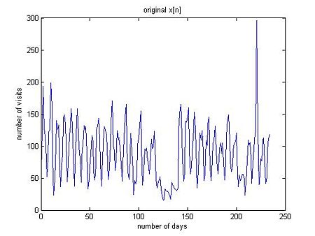
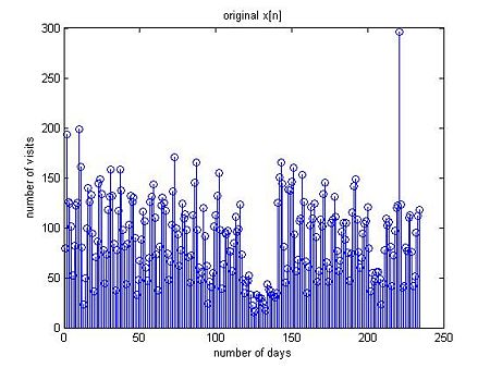
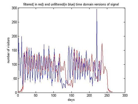
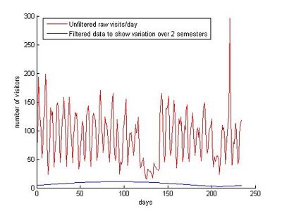
• The number of visits per day from the beginning of fall 2009 to present day was downloaded and the discrete time signal was plotted. Let’s call this signal x[n].If you notice the plot is continuous: this is because there are simply too many points to plot discretely so to prevent getting messy we use the plot command in Matlab instead of stem.
This original x[n] however had too many oscillations for us to get any useful information out of it: we couldn’t tell whether the general traffic increased or decreased over two semesters or remained constant, or what the weekly/monthly variations were.
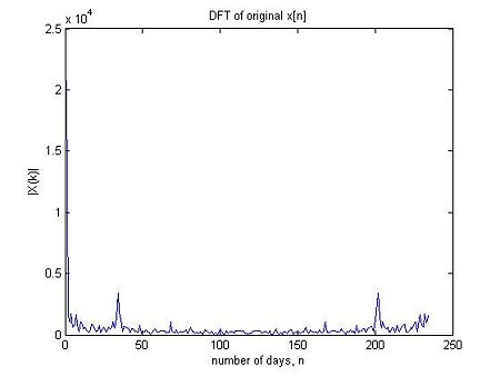
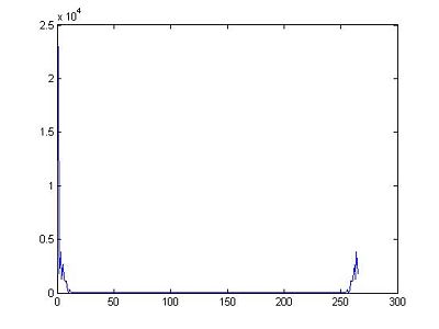
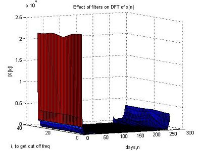
• Therefore a DFT was taken of the x[n] (because the data was discrete and finite in length) and we found that the signal oscillated periodically.As you can see there are peaks at k = 33 and approximately k = 210.This peak at k = 33 corresponds to the weekly variation.
So how do we know that?
Well our signal contains 238 samples for 238 days in total.Earlier I had mentioned that the DFT is almost equal to the DTFT.
$ X(\omega) = X[k] $ if
$ \omega = \frac{k }{N}2\pi $ , for $ k \in \{ 0, 1, \dots, N-1 \} $
N = 238 here. When $ k = 1, \omega = \frac{1}{238} 2\pi $ This corresponds to an event that occurs once every 238 days ---> thus this is the lowest possible frequency of the signal.
The highest possible frequency occurs when k = N i.e. k = 238 which means the event occurs once every day.
Similarly a frequency corresponding to an event that occurs once every seven days ( the weekly variation) = $ \frac{1}{7} 2\pi \simeq \frac{34}{238} 2\pi, k = 34 $
• A low pass filter was then designed with cut off frequencies that represented those weekly variations. A low pass filter is one that passes low frequency signals but attenuates signals that have frequencies higher than the cut off frequency.
Now that we know that k = 34 corresponds to the weekly variation, we need to remove the bump so that we can see the variation over a semester.
Thus our initial cut off frequency,$ \omega_c = \frac{34}{238} 2\pi $
and the filter equation we used was :
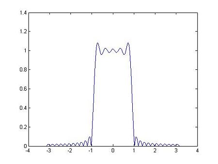
$ h[n] = \frac{\omega_c}{\pi}sinc(\frac{\omega_c}{\pi}(n - \frac{N-1}{2})) $
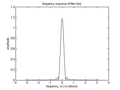
The figure below shows us the impulse response of the filter defined by the equation above.
Note: We could have also used a band pass filter that only removed the k = 32 component rather than removing all the components after k = 32 as the low pass filter does.
The figure below then shows the effect of our low pass filter on the original x[n] in the fourier domain. As you can see the components above k = 32 have all been removed.
It's a pretty cool filter!!!And pretty effective too: a lot of filters have too many side rings that cause a distortion in the signal when the signal and filter are convolved.The filter above also has side rings but not too many ( those tiny bumps after the first zeros on either side are the unwanted side rings called oscillations)
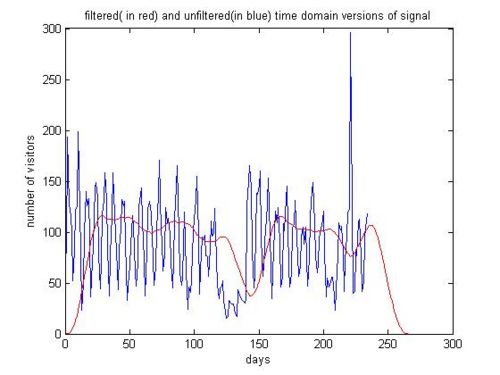
Another low pass filter with $ \omega_c = = \frac{7}{238} 2\pi $ was implemented ( just for the fun of it we took random numbers and tried to see which filter gave us the nicest responses.
NOTE: Did you notice there was a shift in the original x[n] and the filtered x[n]? This is because one of the properties of the DFT is that it is periodic with 2\pi.
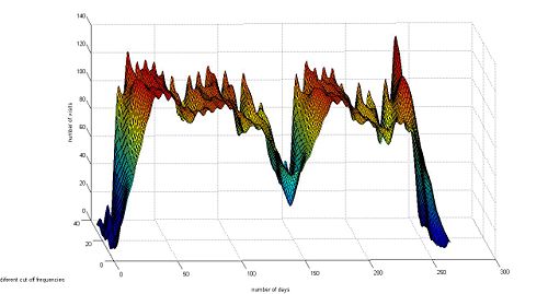
Turns out we can clearly see where the major variations occurred over the period of two semesters.We can account for each those big bumps( or dips) by seeing at what value of k the bump occurred and then translating that k to the nth day in the total of 238 days.Then we can figure out what event ( for example a midterm, or a due assignment) took place on that day.
That really big dip that occurs in the middle of the graph corresponds to the winter break when everyone had gone and no one was really using Rhea.Thus the huge decrease in amplitude. Similarly we can account for other bumps: the other big dips correspond to Thanksgiving and Spring break mostly and the increased usage happened mostly towards the end of the semester when finals were approaching.
Question to be answered from all this: Did Rhea usage generally change over time?
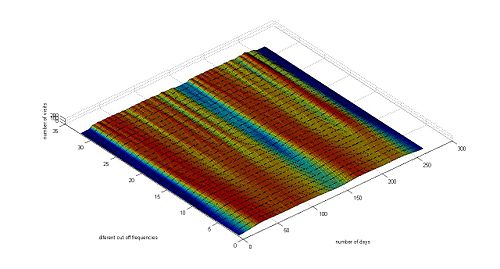
Not really!. It has remained pretty constant (can be seen from the graph below). Monthly variations have also been removed to show this long term trend.
Till now we saw the effects of each filter with its own particular $ \omega_c $ on the signal.
We then created a whole set of low pass filters with $ \omega = \frac{i }{N}2\pi $ , for $ i \in \{ 0, 1, \dots, 32 \} $.
Their collective effect was then noted on the DFT of the signal and its time domain version and then plotted in 3D.
So the above image is like the bird's view of the signal filtered with the same filter but with 32 different cut off frequencies.The blue regions indicate low amplitudes ( on the DFT plot above, the black indicates 0 amplitude) and the red regions indicate the days on which Rhea had the largest number of visitors.
There were some interesting pages that also caused spikes in the visits because of sudden interest generated by pages such as the ones talking about bounties and so on. So money and grades caused increase in usage. So now that we know what (almost) attracts people, we have to set an achievable target to make the website more widespread. This will be done by implementing changes on the website itself and then measure the change in visitor trends. By doing so not only will we increase Rhea’s acceptability and usage but we can also find out what needs to be done to attract people and when certain factors stop functioning as incentives.

