A slecture by Xing Liu
Contents
[hide]Outline of the slecture
- Background in Linear Classifiers
- Support Vector Machine
- Effect of Kernel Functions on SVM
- Effect of Kernel Parameters on SVM
- References
Background in Linear Classifiers
In this section, we will introduce the framework and basic idea of linear classification problem.
In a linear classification problem, the feature space can be divided into different regions by hyperplanes. In this lecture, we take a two-catagory case to illustrate. Suppose we are given training samples
$ \textbf{y}_1,\textbf{y}_2,...\textbf{y}_n \in \mathbb{R}^p $ , where each $ \textbf{y}_i $ is a p-dimensional vector and belongs to either class w1 or w2. The goal is to find the maximum-margin hyperplane that separate the points in the feature space that belong to class w1 from those that belong to class w2. If the data is linear seperable, the discriminate function can be written as
We want to find $ \textbf{c}\in\mathbb{R}^{n+1} $ so that a testing data point $ \textbf{y}_i $ is labelled
We can apply a trick here to replace all $ \textbf{y}'s $ in class w2 by $ -\textbf{y} $, then the above task is equivalent to looking for $ \textbf{c} $ so that
$ \textbf{c}\cdot \textbf{y}>0, ~~ \forall \textbf{y} \in ~new~ sample ~space $ .
You might have already observed the ambiguity of $ \textbf{c} $ in the above discussion: if $ \textbf{c} $ separates data, $ \lambda \textbf{c} $ also separates the data. One solution might be to set $ |\textbf{c}|=1 $. Another solution is to introduce a bias denoted b, and ask
In this scenario, the hyperplane is hence defined by $ \{\textbf{y}: f(\textbf{y})=\textbf{c}\cdot \textbf{y} - \textbf{b}=0\} $ and it divides the space into two, the sign of the discriminant function $ f(\textbf{y}) = \textbf{c}\cdot \textbf{y} - \textbf{b} $ denotes the side of the hyperplane a testing point is on. We notice that the decision boundary by this hyperplane is linear, hence the classifier is called a linear classifier. $ \textbf{c} $ is the normal of the plane lying on the positive side of every hyperplane. $ \frac{b_i}{||c||} $ is the distance from each point $ \textbf{y}_i $ to the hyperplane.
To classify the data is equivalent to setting up a hyperplane, i.e. to find the solution for
where $ \textbf{Y} =\begin{bmatrix} y_1^T \\ y_2^T \\ ... \\ y_n^T \end{bmatrix} $ .
In most cases when n>p, it is impossible to find a solution for $ \textbf{c} $. An alternative approach is to find $ \textbf{c } $ that minimize a criterion function $ J(\textbf{c}) $. There are variant forms of criterion functions. For example, we can try to minimize the error vector between $ \textbf{c}\cdot\textbf{y} $ and $ \textbf{b} $, hence the criterion function is defined as
The solution to the above problem is
otherwise, the solution is defined generally by
This solution is a MSE solution to $ \textbf{Y}\textbf{c} = \textbf{b} $ and it always exists.
Support Vector Machine
Linear SVM
Support vector machine is an example of a linear classifier. For a given hyperlane, we denote $ \textbf{y}_1(\textbf{y}_2) $ the closest points to the hyperpalne among the positive (negative). By geometry the distance from the two points to the hyperplane is $ g(\textbf{y}_1)/||c|| $ and $ g(\textbf{y}_2)/||c|| $. The margin is defined as the region between the two points. In SVM, the hyperplane is chosen so that the margin is maximized, i.e. we want to maximize 1/||c||, which is equivalent to minimizing | | c | | 2. This leads to the following optimization problem:
A more general classifier that allows misclassfication would be
where ξi ≥ 0 are slack variables that allow an example to be in the margin (0 ≤ ξi ≤ 1, also called a margin error) or to be misclassified (ξi > 1). The constant C > 0 sets the relative importance of maximizing the margin and minimizing the amount of slack. Using the method of Lagrange multipliers, we can obtain the dual formulation which is expressed in terms of variables αi:
Nonlinear case
In many applications the data is not linearly separable, in this case 'kernel trick' is applied to map the data into high-dimensional feature spaces. We first map the input space to a feature space using $ \varphi: \mathbb{R}^n \rightarrow \mathbb{R}^m $. Then the discriminant function becomes
Suppose $ \textbf{c} $ can be expressed as a linear combination of the input data points $ \textbf{c} = \sum_{i=1}^{n}\alpha_i\textbf{y}_i $, then the discriminant function in the new feature space takes the form
By defining a kernel function as a mapping function
that satisfies
the discriminant function can be written in terms of the kernel function
The resulting algorithm is formally similar to the linear SVM, except that every dot product is replaced by a nonlinear kernel function.
There are several kernel functions we can choose from. Some common kernels include:
| Linear | $ k(\textbf{x}_i,\textbf{x}_j)=\textbf{x}_i\cdot\textbf{x}_j $ |
| Polynomial | $ k(\textbf{x}_i,\textbf{x}_j) = (\textbf{x}_i\cdot\textbf{x}_j+1)^d $ |
| Gaussian radial basis function | $ k(\textbf{x}_i,\textbf{x}_j) = exp(-\gamma||\text{x}_i-\textbf{x}_j||^2) $ |
To train an SVM and find the large margin hyperplane, one needs to set the parameters αi and $ \textbf{b} $. Other than the parameters in the optimization problem, the SVM has another set of parameters called hyperparameters, including the soft margin constant, C, and any parameters of the kernel function. In the following sections we will apply SVM on classification problem using different kernel functions, then illustrate the effect of the parameters of kernel functions on the SVM classification.
Effect of Kernel Functions on SVM
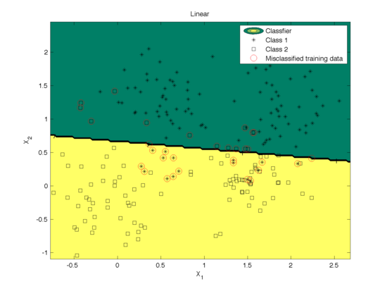
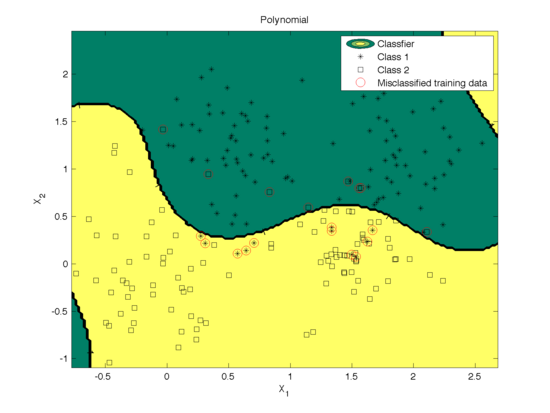
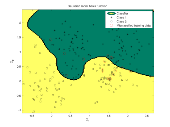
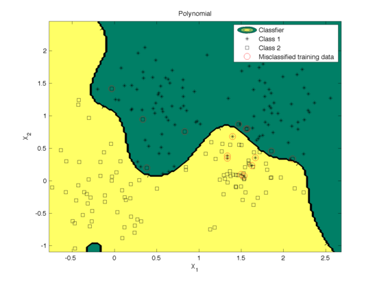
Different kernel functions performs variantly depending on the structure of training data. In the section we give examples of using SVM to classify the Ripley data set (with mixture of two Gaussian distributions in each class) based on the above three kernel functions. The classfications are illustrated in Fig.1~3. The parameters are tuned by cross-validation. The mis-classification rates calculated based on the 10 fold cross validation using the data set are as follows
| Linear | 0.1488 |
| Polynomial | 0.0744 |
| Gaussian radial basis function | 0.0651 |
We can see that in this example when data is not linearly seperable, the polynomial kernel and Gaussian radial basis function work much better than linear kernel functions as expected.
Effect of Kernel Parameters on SVM
You might have noticed the parameters in the kernel functions (width of a Gaussian kernel or degree of a polynomial kernel). The parameter can be tuned using cross-validation to achieve the best performance, which is what we have done in the previous section. In this secion, we manually adjust the parameters to see the effect on the classification.
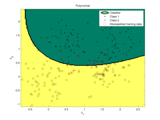
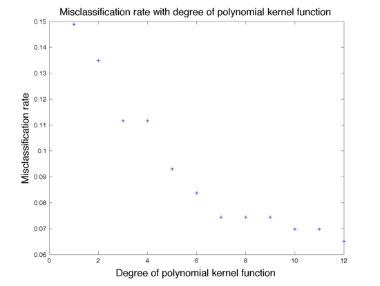
The effect of degree of polynomial kernel function on the classification is shown in Fig. 4. Figure 5 shows the mis-classification rate as a function of the degree. We can see that higher degree polynomial kernels allow a more flexible decision boundary and higher accuracy. For the data set in our example, higher degree also leads to a low mis-classification rate.

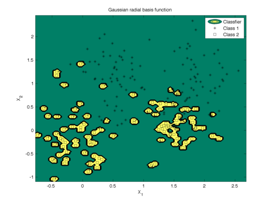
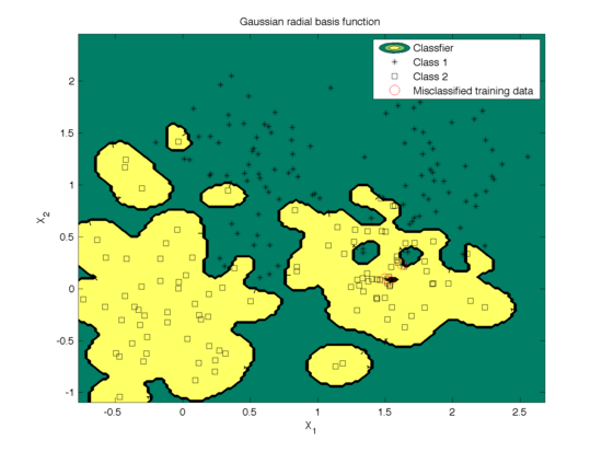
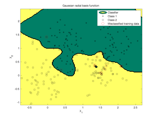
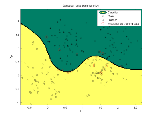
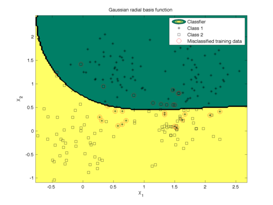
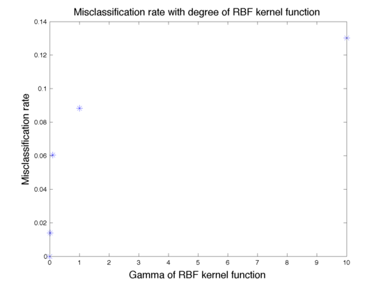
The effect of the width parameter of the Gaussian kernel (γ) is shown in Fig. 6 and the mis-classfication rate is shown in Fig. 7. We can see that for large values (100) of γ the decision boundary is nearly linear. As γ<span class="texhtml"</span> decreases, the flexibility of the decision boundary increases. Small values of γ might lead to overfitting, as shown in the first figure.
References
[1]. Mireille Boutin, "ECE662: Statistical Pattern Recognition and Decision Making Processes," Purdue University, Spring 2014.
[2]. "Pattern Classification" by Duda, Hart, and Stork
[3]. "A User’s Guide to Support Vector Machines" by Ben-Hur and Weston
[4]. LS-SVM lab: http://www.esat.kuleuven.be/sista/lssvmlab/
Questions and comments
If you have any questions, comments, etc. please post them on this page

