Frequency Downsampling - Rhea

Introduction

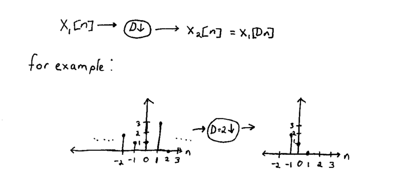
Remember for time domain, Downsampling is defined as:



Now let's describe this process in the frequency domain.

Derivation

First we'll take the Discrete Time Fourier Transform of the original signal and the downsampled version of it.

$ \begin{align} \mathcal{X}_2(\omega) &= \mathcal{F }\left \{ x_2[n] \right \} = \mathcal{F }\left \{ x_1[Dn] \right \}\\ &= \sum_{n=-\infty}^\infty x_1[Dn]e^{-j\omega n} \end{align} $
make the substitution of $ n=\frac{m}{D} $

$ \begin{align} \mathcal{X}_2(\omega) &= \sum_{m=-\infty}^\infty x_1[m]e^{-j\omega \frac{m}{D}} \end{align} $

Downsampled signal will only be nonzero for m equal to multiples of D so:
$ \begin{align} \mathcal{X}_2(\omega) &= \sum_{m=-\infty}^\infty s_d[m]x_1[m]e^{-j\omega \frac{m}{D}} \text{ where}\\ &s_d[m] = \left\{ \begin{array}{ll} 1, & \text{for }m\text{ multiples of } D\\ 0, & \text{else} \end{array} \right.\\ &\text{ or }=\frac{1}{D}\sum_{k=0}^{D-1} e^{jk2\pi \frac{m}{D}} \text{ so:}\\ \mathcal{X}_2(\omega) &= \sum_{m=-\infty}^\infty \frac{1}{D}\sum_{k=0}^{D-1} x_1[m]e^{jk2\pi \frac{m}{D}}e^{-j\omega \frac{m}{D}}\\ &= \frac{1}{D}\sum_{k=0}^{D-1}\sum_{m=-\infty}^\infty x_1[m]e^{-jm\frac{\omega -k2\pi}{D}} \\ \end{align} $

Comparing to
$ \begin{align} \mathcal{X}(\omega) &= \sum_{n=-\infty}^\infty x[n]e^{-jn\omega}\\ \end{align} $

We can rewrite the previous as
$ \begin{align} \mathcal{X}_2(\omega) &= \frac{1}{D}\sum_{k=0}^{D-1} \mathcal{X}(\frac{\omega -2\pi k}{D}) \\ \end{align} $

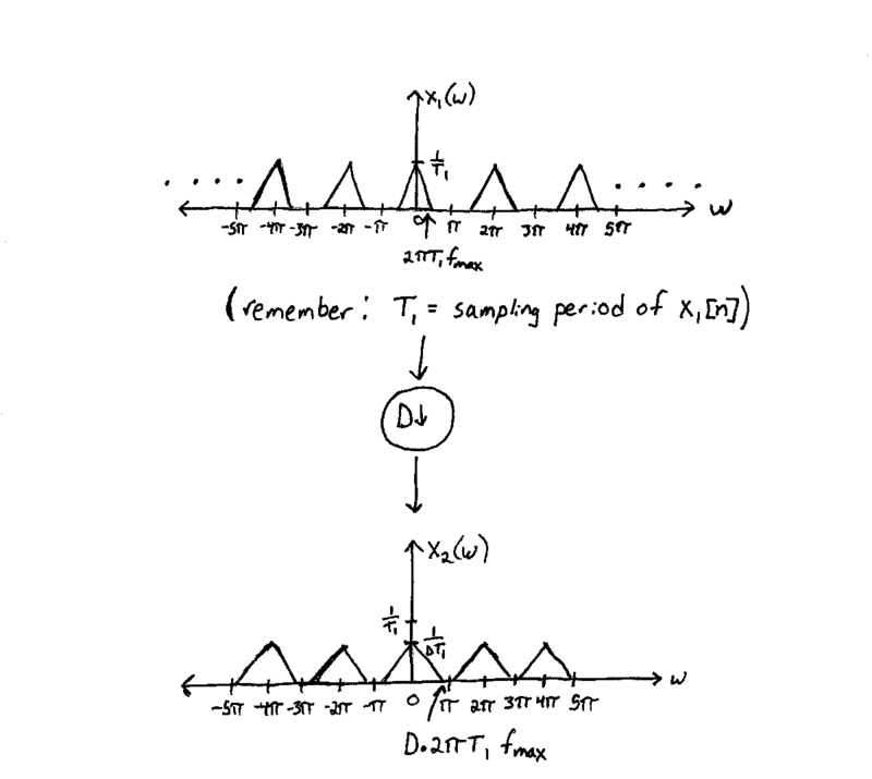
$ \text{Comared to } \mathcal{X}_1(\omega) \text{, } \mathcal{X}_2(\omega) \text{ is } \frac{1}{D} \text{times the magnitude, has its frequencies stretched by }D \text{ and also repeats every }2\pi \text{ (as every DTFT should)} $

Example

It is worth noting that for large enough $ D $ it is possible for the ends of repetitions to overlap, leading to aliasing! To prevent this:

$ \begin{align} D2\pi T_1 f_{max} < \pi\\ \\ x_1[Dn] \text{ has a sampling period of } T_2 = DT_1\text{, so:}\\ \\ \begin{align} \frac{T_2}{T_1}2\pi T_1f_{max} < \pi\\ f_{max} < \frac{1}{2T_2} \end{align} \end{align} $

To make sure this condition is satisfied, we should first pass the original $ x_1[n] $ signal through a low-pass filter with $ f_c = 1/(2T_2) $ BEFORE downsampling.

Since the possible aliasing is caused by the downsampling, trying to low-pass filter after the downsampling will be too late and won't be able to get rid of the aliasing. Thus, the full process of downsampling should look like this:

Conclusion

There are two important points to take away about downsampling's effects in the frequency domain:

1. The downsampled signal's frequency spectrum will have its magnitude lowered by the downsampling factor $ D $, and will repeat every $ 2\pi $
2. Downsampling can cause aliasing. To prevent this, we need to lowpass filter BEFORE the downsampling causes any aliasing.

Questions and comments

If you have any questions, comments, etc. please post them on this page.