- ↳ Topic 3: Magnetic Resonance Imaging
The Bouman Lectures on Image Processing
A Slecture by Maliha Hossain
Topic 3: Magnetic Resonance Imaging
© 2013
Contents
[hide]- 1 Excerpt from Prof. Bouman's Lecture
- 2 Accompanying Lecture Notes
- 2.1 MRI Attributes
- 2.2 Magnetic Resonance
- 2.3 The MRI Magnet
- 2.4 Magnetic Field Gradients
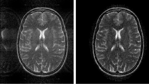
- 2.5 MRI Slice Select
- 2.6 Slice Select Pulse Design
- 2.7 Imaging the Selected Slice
- 2.8 Signal from a Single Voxel
- 2.9 Analysis of Phase
- 2.10 Received Signal from Voxel
- 2.11 Received Signal from Selected Slice
- 2.12 About K-Space
- 2.13 K-Space Interpretation of Demodulated Signal
- 2.14 Controlling K-Space Trajectory
- 2.15 Echo Planar Imaging (EPI) Scan Pattern
- 2.16 Spacing between Readings in EPI Scan Pattern
- 2.17 References
- 2.18 Questions and comments
Excerpt from Prof. Bouman's Lecture
Accompanying Lecture Notes
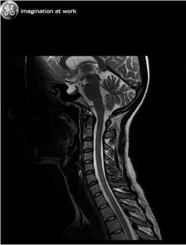
Magnetic resonance imaging (MRI or MR) is a medical imaging technique that uses the property of nuclear magnetic resonance. We will see later in greater detail that magnetic fields are applied to manipulate the precession of nuclei within the patient's body. As the nuclei return to their previous states, they emit a signal that can be decoded into a mapping of the body's internal structure.
There is, in principal, no upper bound to how high the resolution can be of images produced using MRI. It would of course take a long time to perform such a scan. Generally scans have a spatial resolution in the order of millimeters.
Another advantage of MRI is that it uses no ionizing radiation unlike CT. Additionally, MR is very flexible and programmable. It is basically a software programmable module. MR is however about twice as expensive as CT and the duration of the scan is one reason behind the cost. The machine itself is also acoustically noisy, which can be uncomfortable for the patient and can interfere with your measurements if for example you are trying to image the part of the brain that is stimulated by sound.
These notes present a simplified explanation of the physics. A full explanation is beyond the scope of the lecture since it will mainly deal with the signal processing aspect of MRI.
MRI Attributes
- Based on magnetic resonance effect in atomic species
- Does not require any ionizing radiation
- Numerous modalitites
- Conventional anatomical scans
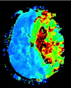
- Functional MRI(fMRI)
- MRI Tagging (tagging makes it possible to capture and store information about the motion of an organ, often of the heart)
- Image formation
- RF excitation of magnetic resonance modes
- Magnetic field gradients modulate resonance frequency
- Reconstruction computed with inverse Fourier transform
- Fully programmable
- Requires an enormous (and very expensive) superconducting magnet
Magnetic Resonance
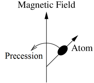
You put a muclear species that has a magnetic dipole in the presence of a magnetic field and this will cause the particle spin to precess about the external field axis much like how a top spins about its axis. This phenomenon is depicted in figure 4.
Larmor precession is the precession of the magnetic moments of atoms or their particles about an external magnetic field.
An atom or its nuclei will precess at the Larmor frequency, given by
$ \omega_0 = LM \ $
where
$ M $ is the magnitude of the ambient magnetic field in Teslas (T)
$ \omega_0 $ is the frequency of precession in radians per second
$ L $ is the gyromagnetic constant known as the Larmor constant and its value depends on the choice of atom. L has units of radians per second per Tesla (rad/(sT))
The Larmor constant is unique to a nuclear species so the frequency of oscillation is intrinsic to a nuclear species in a given magnetic field. Scanners are designed around a particular $ \omega_0 $ depending on which nucleus you are imaging. Typically they are built to image hydrogen ions because of the abundance of these ions, which are essentially protons, in our bodies. The frequency of oscillation of hydrogen in the presence of a magnetic field of 1.5 T is about 63.87 MHz.
Picture initially that the protons are precessing in uniform magnetic field. You introduce more energy into the system via an RF signal at 63.87 MHz. This will cause protons at that frequency to resonate. You have basically pumped energy into the system and the way to describe that is that the tip angle of the precession increases. Once you turn it off, the precessing particle will radiate an RF signal. You can locate the source of the protons by detecting this reradiated RF signal.
As we saw in the previous equation, the Larmor frequency of the detected signal, $ \omega_0 $, is proportional to the applied magnetic field $ M $. Changing the magnitude of that field will produce a different detected frequency. In MRI, a magnetic field gradient across a sample allows you to pinpoint the source of the proton nuclear magnetic resonance (NMR) signal in the sample.
The MRI Magnet
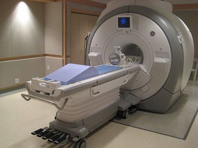
Traditional MR scanners use very high field strengths on the order of 1.5 T and 3 T. these are standard magnetic field strengths and are needed to produce high quality images reliably. Patients are required to remove clothing items that may contain ferromagnetic materials. Most patients with metallic implants such as pacemakers cannot have an MRI done.
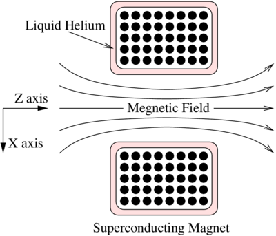
The machine has a large superconducting magnet built around the bore of the scanner. At very low temperatures, close to absolute zero, the superconducting material has zero resistance. A current is passed through the material using a generator. The current continues to pass through it even after the generator is turned off since the material has no resistance for as long as the superconducting material is kept below its critical temperature by the liquid helium.
This perpetual current flow comes at the cost of having to keep the helium cool. An accidental shut-down of the system can trigger an event known as "quench", which involves the rapid boiling of the liquid helium from around the superconducting material. As the temperature rises the magnet develops a resistance and even a small resistance can cause the material to heat up due to the presence of high currents. This will speed up the boiling of the helium even more. If the rapidly expanding helium cannot be dissipated, it may be released into the scanner room, maybe even at an explosive rate. Therefore rooms with scanners must be equipped to handle such an event.
For the remainder of the notes, we will assume the scanner is designed such that $ M_0 = 1.5T $ to image hydrogen ions precessing at 63.8 MHz.
Magnetic Field Gradients
Assume that the direction of the magnetic field within the bore is constant and only its magnitude is changing. This allows us to treat it as a scalar quantity even though in reality it is a vector.
The magnetic field magnitude at the location $ (x,y,z) $ has the form
$ M(x,y,z) = M_0 + xG_x + yG_y + zG_z \ $
- $ G_x $, $ G_y $ and $ G_z $ control magnetic field gradients
- $ M_0 $ is constant.
So the equation is basically saying that a constant magnetic field, $ M_0 $ is applied to the entire sample. The hydrogen spin-flip frequency is then the same for all parts of the sample. Then you add variable magnetic fields using gradient coils that are controlled by amplifiers. These coils are similar to ones in your speaker systems. The coils are designed so that the magnetic field changes approximately linearly with position, hence the term gradient field.
In other words, you have the static uniform magnetic field $ M_0 $ produced by the superconducting magnet. Add to this the gradient magnetic field that varies linearly with space. The gradient field is produced by a current through a coil driven by an amplifier. It is important to note that the gradients can be changed with time and that they are small compared to $ M_0 $.
For the inductance $ L $ in the coil, we know that
$ L\frac{di}{dt} = v(t) $
Recall from Ampere's law that the magnetic field around an electric current is proportional to the current. The magnetic field is therefore also proportional to the integral of the voltage across the coil
$ M(t) = \int v(\tau)d\tau $
The amplifier that drives the current through the coil is controlled by a voltage where the current through the coil is proportional to the integral of the voltage and the magnetic field of the coil is proportional to the current.
For the time varying gradients,
$ M(x,y,z,t) = M_0 + xG_x(t) + yG_y(t) + zG_z(t) \ $
The three coils produce gradients along $ x $, $ y $ and $ z $ (left to right, top to bottom and head to toe respectively). Each of those coils control the magnetic field gradient along its respective axis. So by varying the current through each of those three coils, the gradient field can be varied along each axis.
MRI Slice Select
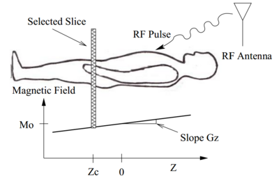
Let us consider the $ z $ axis along the bore. The graph for $ M $ versus $ z $ is a straight line with gradient $ G_z $ so as you move from the toes towards the head, the magnetic field increases. Now if you send an RF pulse at 63MHz you can excite protons inside the patients body but only for those where the resonant frequency matches the RF frequency.
As shown in the figure, the magnetic field is equal to M_0 at $ z = 0 $ therefore, the protons on this plane have precession frequency 63MHz. These protons will resonate with the RF pulse that is transmitted at 63MHz. RF is not much attenuated by the patient's body. At each position, the atoms are tuned to a different frequency. By varying the frequency of the RF pulse, you could stimulate protons from different slices along the z-axis. In this manner you could specify which slice to stimulate, hence the term slice select.
Here is a summary of the strategy behind slice select:
Design RF pulse to excite protons in single slice
- Turn off $ x $ and $ y $ gradients
- Set $ z $ gradient to fix positive value, $ G_z > 0 $
- Use the fact that resonance frequency is given by $ \omega = L(M_0+zG_z) $
Slice Select Pulse Design
If the RF pulse is a sinc function modulated at 63.8 MHz, its Fourier transform would be a shifted rect. This would essentially be a slice in the frequency domain whose width is governed by the width of the sinc. A wider sinc would produce a narrower slice. In this manner, you could gather a sequence of slices that fit next to each other to build up a 3 dimensional representation of the volume.
So to summarize, you would need to consider the following parameters in designing your RF pulse:
- Slice center$ = z_c $, governed by the carrier frequency
- Slice thickness $ = \Delta z $, governed by the width of the sinc function.
To image the slice centered at $ z_c $, the pulse frequency is given by
$ f_c = \frac{LM_0}{2\pi}+\frac{z_cLG_z}{2\pi} = f_0 + \frac{z_cLG_z}{2\pi} $
The slice thickness $ \Delta z $ can be used to calculate the pulse bandwidth
$ \Delta f = \frac{\Delta z LG_z}{2\pi} $
Using the parameters, the pulse is given by
$ s(t) = e^{j2\pi f_ct}sinc(t\Delta f) $
and its CTFT is given by
$ S(f) = rect(\frac{f-f_c}{\Delta f}) $
Imaging the Selected Slice
When the duration of the pulse is over, precessing atoms will reradiate electromagnetic energy at RF frequencies as they relax. Below is an overview of the strategy used to image a slice:
- Vary magnetic gradients along $ x $ and $ y $ axes. The magnetic field varies approximately linearly with respect to position.
- Measure the received RF signal
- Reconstruct an image from the RF measurements.
Signal from a Single Voxel
Let us first analyze the signal received from one voxel. In our given coordinate system, this voxel is of size $ dxdydz $. Then we can look at the signal we would get from adding all the voxels together. We do this by integrating across all of them to obtain the total signal received at the antenna.
Assume that we have selected a slice on the $ z $-axis so the received signal is a function of $ x $, $ y $ and time.
The RF signal from a single voxel has the form
$ r(x,y,t) = f(x,y)e^{j\phi(t)} \ $
$ f(x,y) $ is a voxel dependent weighting where $ f(x,y) $
- depends on properties of material in voxel
- is the quantity of interest
- typically "weighted" by T1, T2, or T3*
The received signal has phase $ \phi(t) $. This phase terms appears due to the fact that the linear gradients have been changed at this point. The real part of $ f(x,y)e^{j\phi(t)} $ is what you receive at the antenna but it is standard to include the expression for phase in a modulated signal. By modulation, I mean that a sinusoidal carrier, which can be expressed as a complex exponential, is multiplied with your original signal
The phase can be modulated using $ G_x $ and $ G_y $ magnetic field gradients. You can employ the gradients to pinpoint a single voxel in a slice. If the voxel is at $ (z=z_0, x=0, y=0) $ changing the gradient will not matter but elsewhere in the slice, it will.
Without loss of generality, we assume that $ \phi(0) = 0 $. In doing do, we absorb any complex constant into $ f(x,y) $ so that $ f(x,y) $ can be a complex number. By changing the gradient along $ x $ and $ y $, you can manipulate the oscillation frequency of that voxel.
For a signal given by $ e^{j\phi(t)} $, the phase is given by $ \phi(t) $. The instantaneous frequency $ f(t) $, is the time derivative of the phase i.e.
$ \begin{align} f(t) &= \frac{d\phi(t)}{dt} \\ \Rightarrow \phi(t) &= \int_{-\infty}^t f(\tau) d\tau \end{align} $
Analysis of Phase
Recall that the oscillation frequency is given by $ \omega_0 = LM $. And we have also just covered that the instantaneous frequency is the time derivative of phase. Therefore
$ \begin{align} \frac{d\phi(t)}{dt} &= LM(x,y,t) \\ \Rightarrow \phi(t) &= \int_0^t LM(x,y,\tau)d\tau \\ &= \int_0^t LM_0 + xLG_x(\tau) + yLG_y(\tau)d\tau \\ &= \omega_0t + xk_x(t) +yky(t) \end{align} $
where we define
$ \omega_0 = LM_0 $
$ k_x(t) = \int_0^t LG_x(\tau)d\tau $
$ k_y(t) = \int_0^t LG_y(\tau)d\tau $
So the phase is the nominal frequency times $ t $ plus the $ xk_x(t)+yk_y(t) $, which is the phase shift due to the gradient magnetic fields along $ x $ and $ y $.
The RF signal reradiated by a single voxel has the form
$ \begin{align} r(t) &= f(x,y)e^{j\phi(t)} \\ &= f(x,y)e^{j(\omega_0t + xk_x(t) + yk_y(t))} \\ &= f(x,y)e^{j\omega_0t}e^{j(xk_x(t) + yk_y(t))} \end{align} $
Note that the $ \phi(t) $ is not expressed as a function of $ z $. This is because we have restricted ourselves to one slice on the $ z $ axis so in this analysis, the value of $ z $ does not vary.
Received Signal from Voxel
From the above analysis of phase, we have that the received RF signal from a single voxel is given by
$ \begin{align} r(t) &= f(x,y)e^{j\phi(t)} \\ &= f(x,y)e^{j(\omega_0t+xk_x(t)+yk_y(t))} \\ &= f(x,y)e^{j\omega_0t}e^{j(xk_x(t)+yk_y(t))} \end{align} $
where $ e^{j\omega o(t)} $ is the carrier and $ e^{j(xkx(t)+yky(t))} $ is the phase modulation on the carrier. In order to demodulate the signal in the receiver, the signal $ r(t) $ is fed into a mixer where it is multiplied with the reciprocal of the carrier and you are then left with the image multiplied with the phase modulator as shown in figure 9.
Received Signal from Selected Slice
The RF signal from the complete slice is given by summing the contributions from all the voxels in that slice so we integrate over $ x $ and $ y $ to get
$ \begin{align} R(t) &= \int_{\mathbf{R}}\int_{\mathbf{R}}r(x,y,t)dxdy \\ &= \int_{\mathbf{R}}\int_{\mathbf{R}} f(x,y)e^{j\omega_0t}e^{j(xk_x(t) + yk_y(t))}dxdy \\ &= e^{j\omega_0t}\int_{\mathbf{R}}\int_{\mathbf{R}} f(x,y)e^{j(xk_x(t) + yk_y(t))}dxdy \\ &= e^{j\omega_0t}F(-k_x(t),-k_y(t)) \end{align} $
where $ F(u,v) $ is the CSFT of $ f(x,y) $, $ u = -k_x(t) $ and $ v = -k_y(t) $
So we have that the demodulated received signal $ R(t)e^{-j\omega ot} $ is the Fourier transform of the object evaluated at $ -k_x(t) $ and $ -k_y(t) $.
About K-Space
K-space is simply an array of numbers representing the MR signals. We can use these values to recreate the MR image. The k in k_space refers to the wave number, or the number of wave cycles per meter of linear space. This is a notation commonly used in physics but it is easily converted to frequency if you note that $ \omega = 2\pi k $.
k-space is the plot of wave numbers but you can also think about it in frequency. Really the domain of the k-space is a 2 dimensional frequency domain. Signals with the same wave number or frequency must still be distinguishable if they have different phases. For this reason, the range of the k-space is complex.
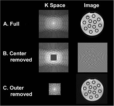
Every value in the array represents a wave of some frequency, amplitude and phase. If we superimpose all these waves we can form the MR image. Contrast information, appearing in large areas of bright an dark, is contained in the lower spatial frequencies. High spatial frequencies contain detail and edge information. This is illustrated in figure 10.
K-Space Interpretation of Demodulated Signal
Demodulating the RF signal from the complete slice, we get
$ F(-k_x(t),-k_y(t))=R(t)e^{j\omega_0t} $
where
$ k_x(t) = \int_0^t LG_x(\tau)d\tau $
$ k_y(t) = \int_0^t LG_y(\tau)d\tau $
Strategy
- Scan partial frequencies by varying $ k_x(t) $ and $ k_y(t) $
- Reconstruct image by performing the (inverse) CSFT
- $ G_x(t) $ and $ G_y(t) $ control velocity through K-space
Controlling K-Space Trajectory
Relationships between gradient coil voltage and K-space:
$ \begin{align} L_x\frac{di(t)}{dt} &= v_x(t) \quad G_x(t) = M_xi(t) \\ L_y\frac{di(t)}{dt} &= v_y(t) \quad G_y(t) = M_yi(t) \end{align} $
where $ v_x(t) $ and $ v_x(t) $ are the voltage across the respective coils and $ L_x $ and $ L_y $ are their respective inductances.
Using this result, we get
$ \begin{align} k_x(t) &= \int_0^t LG_x(\tau)d\tau \\ &= \frac{LM_x}{L_x}\int_0^t\int_0^{\tau}v_x(s)dsd\tau \\ k_y(t) &= \int_0^t LG_x(\tau)d\tau \\ &= \frac{LM_y}{L_y}\int_0^t\int_0^{\tau}v_y(s)dsd\tau \end{align} $
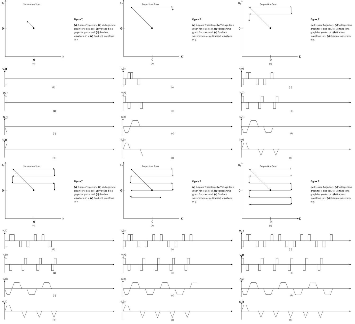
$ v_x(t) $ and $ v_y(t) $ are like the accelerator peddles for $ k_x(t) $ and $ k_y(t) $ in the professors force-displacement analogy and $ G_x(t) $ and $ G_y(t) $ are like analogous to velocity. This concept is further illustrated in figure 10.
Assume that a particle is at rest at position $ (x=0,y=0) $ on the grid shown in figure 10. A negative acceleration pulse is applied along the $ x $-axis and a positive acceleration pulse is applied along the $ y $-axis, so that the particle travels to the top left corner of the grid. The particle is brought to a stop with another pulse in the opposite direction. Next a pulse is applied along the positive $ x $-axis and the particle travels to the top right of the grid, where it is stopped and made to travel downward due to a negative acceleration along the $ y $-axis. The pulses are applied so that the particle travels from the top left to the bottom right corner of the grid in a serpentine path. The full sequence is illustrated in figure 10. But really acceleration is an analogy for voltage and the velocity is an analogy for $ G_x(t) $ and $ G_y(t) $. $ k_x(t) $ and$ k_y(t) $ are analogous to displacement along the $ x $ and $ y $ axes. The voltage waveforms required to trace such a path are shown in figure 10 (d) and (e).
Echo Planar Imaging (EPI) Scan Pattern
Note that I have included what the pulse must look like to move the point from its initial position at the origin to the top left corner of the grid.
Recall that the gradient is proportional to current, which in turn is proportional to the integral of the voltage with respect to time.
$ \begin{align} k_x(t) &= L\int_0^t G_x(\tau)d\tau = \frac{LM_x}{L_x}\int_0^t\int_0^{\tau} v_x(s)dsd\tau \\ k_y(t) &= L\int_0^t G_y(\tau)d\tau = \frac{LM_y}{L_y}\int_0^t\int_0^{\tau} v_y(s)dsd\tau \end{align} $
Spacing between Readings in EPI Scan Pattern
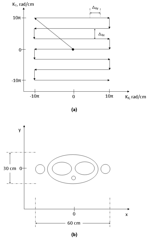
Since the data we have collected is in the frequency domain, we must take the inverse Fourier transform to obtain the real image. Recall that stretching in the frequency domain produces higher resolution in the space domain and vice versa. By scanning across a wide area, we can obtain very high resolution images. You may be tempted to speed this up by increasing the spacing between two horizontal lines shown in figure 11a but we must take care that the spacing between collected data points is small otherwise your field of view shrinks. So if you are imaging a large object, you must ensure that enough data points are collected in the k-space to produce an image that is of adequate size.
The units in the k-space are radians per unit distance, typically centimeters or millimeters. If you were trying to image the 60 cm by 30 cm area shown in figure 11b, what would the maximum spacing between readings have to be in order to reconstruct the image? The highest frequency along each of the axes is 1 mm$ ^{-1} $. What is the area across which you would have to perform the scan in order to achieve this resolution?
Recall from Nyquist sampling theorem, a function that is bandlimited by frequency $ \omega_{max} $ can theoretically be perfectly reconstructed from a countable sequence of samples as long as it is sampled at a rate higher than twice $ \omega_{max} $.
If the highest frequency in your image is 1 mm$ ^{-1} $ or 10 cm$ ^{-1} $, then your sampling frequency, $ f_s $ must be greater than twice this number.
$ \Rightarrow |K_{x,max}| = 2\pi \times \frac{f_s}{2} = 10\pi \; rad/cm $
Similarly,
$ \Rightarrow |K_{y,max}| = 2\pi \times \frac{f_s}{2} = 10\pi \; rad/cm $
Notice that the smaller the voxel, the larger the area that needs to be scanned. The dual nature of the Fourier transform dictates that if you increase the spacing between samples in the space domain, you decrease the bandwidth required to represent the image in the frequency domain and vice versa. If you increase the sample spacing in the frequency domain, your field of view in the space domain decreases. In this scenario, the k-space must be at least $ 20\pi $ rad/cm by $ 20\pi $ rad/cm.
For a 30 cm high field of view, the step size along $ k_x $ is (1/30 × 1/2 × 2π) = π/30 radians per cm. Using a similar argument, we see that the step size along $ k_y $ must be at most (1/60 × 1/2 × 2π) = π/60 radians per cm. aliasing figure 12
Figure 12 illustrates what the effects of aliasing look like. Too few samples were taken along the $ K_x $ axis.
References
- C. A. Bouman. ECE 637. Class Lecture. Digital Image Processing I. Faculty of Electrical Engineering, Purdue University. Spring 2013.
- C. R. Nave. “Nuclear Magnetic Resonance". Internet: http://hyperphysics.phy-astr.gsu.edu/hbase/nuclear/nmr.html, [June 16, 2013].
- Waisman Laboratory for Brain Imaging and Behaviour. "MRI Facilities". Internet: http://brainimaging.waisman.wisc.edu/facilities/MRI.html, May 14th, 2009, [July 14th, 2013].
- G. Francis. Psy 200. "Introduction to Cognitive Psychology". Class Lecture Notes. Faculty of Psychological Sciences, Purdue University. Spring 2013.
- L. Lejeune. "Linear Estimation in Magnetic Resonance Imaging (MRI) - Comparisons of Reconstruction Methods of Images". in Student Projects, École Polytechnique Fédérale de Lausanne. December 1st, 2009.
- D. M. Higgins, "The What is K-Space? Tutorial". Internet: http://www.revisemri.com/tutorials/what_is_k_space/, [July 22nd, 2013]
Questions and comments
If you have any questions, comments, etc. please post them on this page
Back to the "Bouman Lectures on Image Processing" by Maliha Hossain

