Curse of Dimensionality - Rhea

Version of this page in Chinese

Needle in a Haystack

You lost your needle in a haystack. If the world you live in has just one dimension, then you are lucky because the haystack is a line segment. Finding the needle only requires you to start from one end of the segment, heading towards the other end until hitting the needle:

Not bad, right? If you are a 2D creature, a needle in a haystack now becomes a small trouble because it can be any point in a square:

There is much more space for the possible location: within the haystack, the needle can move along either the $ x $-axis or the $ y $-axis. Things get worse and worse as the number of dimensions grows. You can't imagine how alien high-dimensional creatures would look for something missing in their world because even in three dimensions, this task turns out to be frustrating (from everyday life experience):

The difficulty of finding the needle starting from a certain point in a high-dimensional haystack implies an import fact: the points tend to distribute more sparsely (i.e., they are more dissimilar to each other) in high-dimensional space, because the Euclidean distance between two points is large as long as they are far apart in the direction of at least one dimension, even though they may be quite close in the direction of all the other dimensions. This fact can be further illustrated quantitatively by the following example. In $ N $-dimensional space, suppose we want to count all the neighbors around a central point within a hypercube with the edge length equal to 1. We also consider a bigger hypercube around the central point with the edge length equal to $ 1+2\epsilon $, i.e., the smaller hypercube is nested inside the bigger one. As a special case, in 3D space we have the following scenario:

Now if by assumption the points are evenly distributed in the space, then the ratio of the number of the points in the smaller hypercube to the number of the points in the bigger hypercube is given by

 $  (\frac{1}{1+2\epsilon})^N  $

If we take $ \epsilon=0.01 $, then for $ N= $1,2,3,5,10,100, and 1000 we have the ratio equal to 0.98, 0.96, 0.94, 0.91, 0.82, 0.14, and $ 2.51\text{e}^{-09} $. It can be seen that when $ N >= 10 $, the neighbors around a given point become so few that nearly all points are located inside the $ \epsilon $-shell around the smaller hypercube. To maintain a certain number of neighbors, exponentially many new points should be added into the space.

Curse of Dimensionality

Math theorems can often generalize from low dimensions to higher dimensions. If you know how to compute gradients for a function with two variables, then you probably can also figure out how to do that for multi-variable functions. However, this is not the case when you try to generalize your two-dimensional density estimator to hundreds or thousands of dimensions. Theoretically, your estimator should still work in high dimension. But that requires you to collect an exponential number of training data to avoid sparsity. In practice, the available training data are often quite limited.

Your two-dimensional estimator stops working in high dimension because the limited training data in your hand are not statistically significant due to their sparsity, i.e., there is not enough information for you to recover the true underlying distribution. The concept of statistical significance can be illustrated in the one dimensional case as follows. Suppose you are drawing some points from a normal distribution and trying to estimate its parameters. It makes a big difference between if you draw just 10 points and if you draw 100 points from the distribution.

In the above, the first one is the true underlying normal distribution. The second one is being estimated from 10 points. The third one is being estimated from 100 points. Insufficient training points result in a poor estimation.

The curse of dimensionality describes a scenario in which you can't possibly obtain an exponential number of training points in high dimensional space which is just like that somehow after being cursed in the 1D world you can't easily obtain over 10 training points in the above example, thus resulting in high difficulty of reliably estimating density function. This difficulty also arises in seeking a decision boundary between classes using a discriminative classifier. You never know whether the boundary drawn to separate the training points just barely separates some special training samples from the whole population or actually generalizes well to other data. The lack of ability to reliably estimate and generalize is called overfitting. Even with enough training data in low dimensional space, overfitting can still exist due to various reasons (e.g., high model complexity, incorrect collection of training data, etc). However, in high dimensional space, overfitting is more likely to happen because of the lack of training data.

There are several ways to break the curse:

• feature extraction: Most people don't realize that they are actually dealing with the curse of dimensionality in their daily work. No one will directly use all the pixel intensities in an image as the input to their face recognition algorithm. It's simply because there is too much redundant information in that. For example, if you have a 100x100 image, then the raw vector of intensities has a length of 10000! However, if you use the edge pixels or corner points extracted from the image, the dimensionality can be reduced to as small as hundreds or even dozens, with only a small amount of information lost. Because of this reason, lots of people in machine learning and statistics work on the extraction/selection of features. Sometimes it requires prior knowledge to decide on good features.

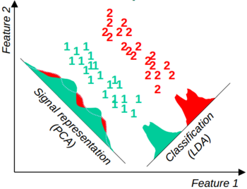
• dimensionality reduction analysis: People came up with statistical methods to automatically reduce the dimensionality. Depending on different criteria, these methods usually have very different reduction results. If the goal is to represent the original high dimensional data in low dimensional space losing as little information as possible (signal representation), then the components that have the largest variance in feature values within classes are kept, which is known as Principle component analysis (PCA). If the goal of reduction is to discriminate different classes in low dimensional space, then the components containing feature values that have the best separation across classes are kept, which is known as Linear discriminative analysis (LDA). The following figure (borrowed from reference 2) shows the difference between the two methods.

• kernel: The needle in a haystack example shows that points tend to be outliers in high dimensional space. Dealing with those points directly is lots of pain. Kernel trick used by support vector machines (SVMs) implicitly maps data to much higher or even infinite dimensions but without ever explicitly representing the high dimensional features. The mapping makes the data that are not linearly separable in low dimensional space linearly separable in high dimensional space (which is also why people want to use many different features). While the classifier learns the decision boundary in a very high dimensional feature space, it actually deals with low dimensionality.

None of the above spells is a complete cure for the curse of dimensionality. There are still many open problems on this topic.

References

1. http://en.wikipedia.org/wiki/Curse_of_dimensionality
2. http://courses.cs.tamu.edu/rgutier/cs790_w02/l5.pdf

Questions and comments

If you have any questions, comments, etc. please post them on this page.

Back to ECE662, Spring 2014