Bayes Parameter Estimation with examples - Rhea

Bayesian Parameter Estimation with examples

A slecture by ECE student Yu Wang

Partly based on the ECE662 Spring 2014 lecture material of Prof. Mireille Boutin.

Introduction: Bayesian Estimation

First recall that the joint probability density function of $(\mathbf X,\theta)$ is the mapping on $S \times \Theta$ given by

(x, \theta) \mapsto \pi(\theta) f(x \mid \theta)

Next recall that the (marginal) probability density function f of $$ X $$ is given by

f(x) = \sum_{\theta \in \Theta} \pi(\theta) f(x | \theta), \quad x \in S

if the parameter has a discrete distribution, or

f(x) = \int_\Theta \pi(\theta) f(x| \theta) \, d\theta, \quad x\in S

if the parameter has a continuous distribution. Finally, according to Bayes rule, the conditional probability density function of $\theta$ given $$ X= x $$ namely posterior is

h(\theta \mid x) = \frac{\pi(\theta) f(x \mid \theta)}{f(x)}; \quad \theta \in \Theta, \; x\in S

Our BP estimator is defined as posterior mean $E(\theta \mid x)$ .

Bayesian Parameter Estimation: Bernoulli Case with Beta distribution as prior

The probability density function of the beta distribution, where $0 \le x \le 1$ , and shape parameters $\alpha,\beta > 0$

f(x;\alpha,\beta) = \frac{1}{ B(\alpha,\beta)} x^{\alpha-1}(1-x)^{\beta-1}

Recall that the Bernoulli distribution has probability density function (given p)

g(x \mid p) = p^x (1 - p)^{1-x}, \quad x \in \{0, 1\}

So, with n i.i.d. samples, the likelihood function will be:

l(\mathbf{X} \mid p) = p^{\sum{x_i}} (1 - p)^{n-\sum{x_i}}, \quad x \in \{0, 1\}

Thus, the posterior, according to Bayes rule,

posterior(p \mid \mathbf{X}) = Cp^{Y+\alpha -1} (1 - p)^{n-Y+\beta-1}, \quad x \in \{0, 1\}

where $Y=\sum{x_i}$ and C is just a scaling constant.

Therefore, $\mathbb{E}(p \mid X) = \frac{\alpha+Y}{\beta+Y+n}$

Bayesian Parameter Estimation: Example

The objective of the following experiments is to evaluate how varying parameters affect density estimation:

1. 1D Binomial data density estimation when varing the number of training data

2. 1D Binomial data density estimation using different prior distribution.

3. 2D synthetic data density estimation when updating our prior guess.

The 1D Binomial test is based on flipping a biased coin. The probabilty that the biased coin appears head is assumed as p, so that the probability of tail is 1-p. In this experiment, we introduce another well-known estimator, maximum a posteriori probability (MAP) estimator. The reason of introducing MAP in the context of comparing MLE and BPE is that MAP can be treated as an intermediate step between MLE and BPE, which also takes prior into account. Note that we can simply define MAP as follows:

\hat{\theta}_{\mathrm{ML}}(x)= \underset{\theta}{\operatorname{arg\,max}} \ f(x | \theta)

First of all, we will examine how the number of training data will affect BPE, MLE and MAP. My question is which one will be the best when our training data is insufficient. To answer this question, we formulate the problem of flipping a biased coin in the following way:

1. number of training data varies from 5 to 200 in step of 10

2. for each case, we use the same prior knowledge, that is $\theta$ follows a Beta distribution(mean = 2/3)

3. for each case, we account 30 trials, which will give us a reasonable mean and variance, where the ground truth of p is 2/3.

Remember that the probability density function of the beta distribution we discussed above.

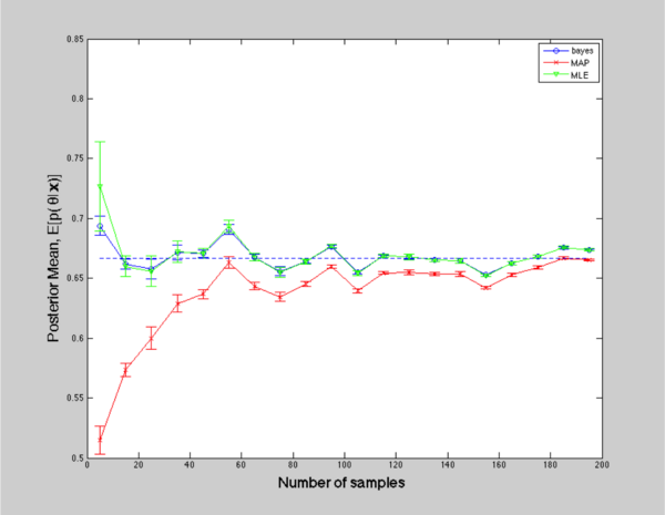
Figure 1: Posterior mean with increasing number of samples

In Figure 1, all curves converge to the true mean as number of training data increases. However, when number of samples is not enough, BPE gives us a better estimation, because it takes all prior information into account, whereas MAP has a huge offset even though it also includes some prior information. The performance of MLE is somewhere between BPE and MAP from the perspective of mean value.

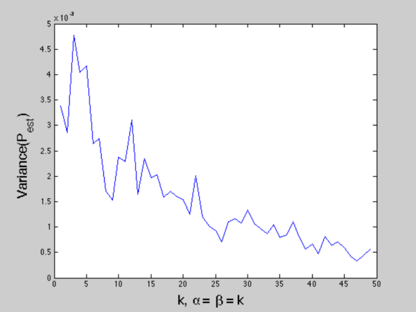
$Figure 2:Variance of $ \hat{p} $ with different prior information$

Figure 2: Variance of $\hat{p}$ with different prior information

If we take a closer look at the variance of each case, we can see that MLE tends to have a larger variance specially when number of samples are insufficient, which means MLE has more uncertainty over what it tries to estimate. On the other hand, BPE and MAP have smaller variance because the prior information limits the uncertainty to a certain range. We can infer that if our prior distribution has a narrower peak at the true mean rather than Beta distribution with a wide ramp, the estimated variance will much smaller.

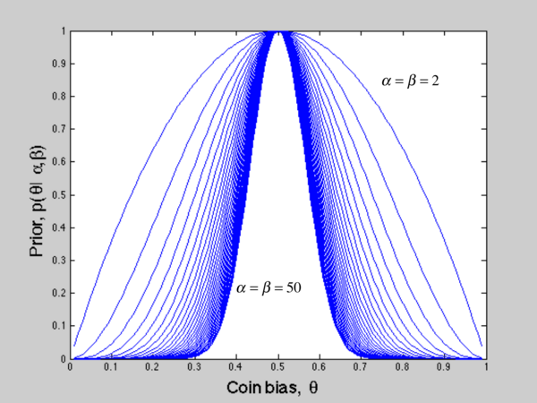
$Figure 3:Beta distribution when varying $ \alpha,\beta $$

Figure 3: Beta distribution when varying $\alpha,\beta$

Figure 2 proves our inference above. In this case, we tempararily let Beta distribution have true mean equal to 0.5 and manipulate two parameters( $\alpha \; and\; \beta$ ) to give us different variance, which represents the uncertainty of our initial guess. Figure 3 shows how Beta distribution changes when using different parameter. Back to Figure 2, we can conclude that certainty of prior knowledge determines the variance of our estimation.

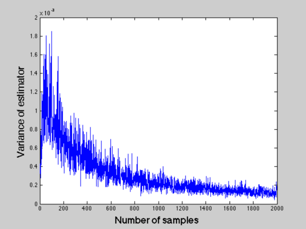
$Figure 4:Variance of $ \hat{p} $ with increasing number of samples$

Figure 4: Variance of $\hat{p}$ with increasing number of samples

You may also ask how the number of samples affect the variance. Figure 4 tells us that starting from a really small number of samples, 5 in our case, the variance tends to go up and then go down to zero. The reason of such phenomenon is that when number of samples is so small, the prior is dominant so that the estimation is simply a reflection of prior, which tends to have a small variance.

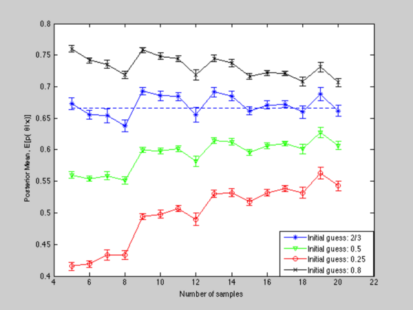
Figure 5: Posterior mean with different initial guess

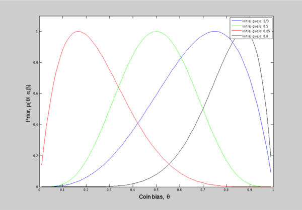
Figure 6: Prior: Beta distribution with various parameters

Now, let's discuss what if our prior knowledge is biased, say the true mean is 0.6, but we model our prior as a gaussian centered at 0.2. Still using the problem we formulated before, where our ground truth is 2/3, we force our prior to be biased. As Figure 5 and Figure 6 shows, four initial guesses are implemented for a relatively small amount of samples. We can see that results from different prior knowledge vary a lot and the effect of prior is dominant in this case. With more data, such effect will be attenuated and the influence of data will be essential then. Figure 7 simply shows how posterior updates according to different prior.

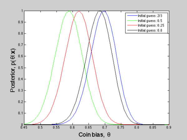
$Figure 7:Posterior: likelihood $ \times $ prior$

Figure 7: Posterior: likelihood $\times$ prior

Secondly, I will discuss how to update prior in a recursive way to reach a better estimation. In this experiment, assume there is an intruder UFO detected by global radar in the year of 2050. With advanced technology, the UFO can produce Gaussian noise over its position to illude our radar. However, aliens don't know we have learned Bayes Estimation.

For simplicity, we limit the detection of UFO in a certain range[3:5,4:6] and the true location is [3.5,4.5], which is unknown to us. What we know from our military radar is shown in Figure 8. The illusions that aliens created follow gaussian distribution with standard deviation of 2 centered at true location.

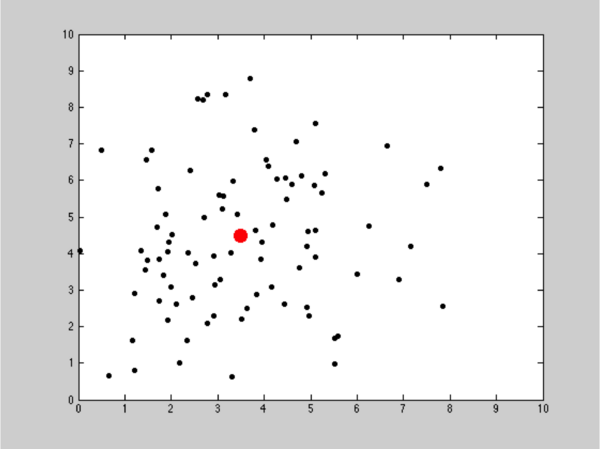
Figure 8: UFO location on radar

To start off, our initial guess is just a unform distribution in the region we limit. In this case, we have 100 observations on our radar. From each observation, we update the prior according to previous posterior. Figure 9 illustrates three stages of our detection. As we can see, with more data collected, our prior information is more constrained. In another word, the confidence of detection is growing with observations.

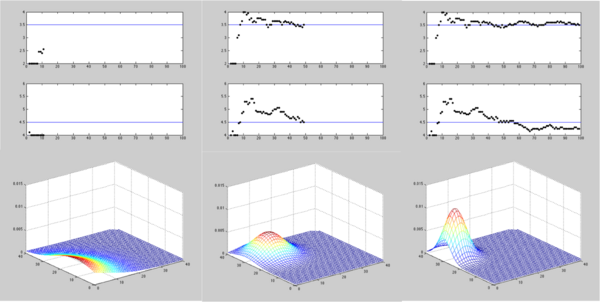
Figure 9: Updating prior with data: first line represents X,Y coordinates, second line is the updated prior distribution

References

[1]. Mireille Boutin, "ECE662: Statistical Pattern Recognition and Decision Making Processes," Purdue University, Spring 2014.

[2]. Virtual Laboratories, "Virtual Laboratories in Probability and Statistics"

Questions and comments

If you have any questions, comments, etc. please post them on this page.

Back to ECE662, Spring 2014