PageRank Algorithm
Let us understand the Page Rank Algorithm through an example. We use a simplified version of it, which only considers connected graphs. In real life, we could have disjoint sets of websites. Our focus of the algorithm is its linear algebra perspective.
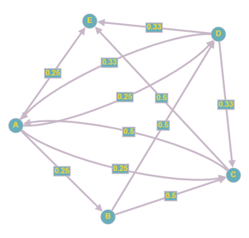
Suppose we have a smaller version of the internet of websites A, B, C, D, E as described in the table below.
| Website | Links to Website(s) |
|---|---|
| A | B, C, D, E |
| B | C, D |
| C | A, E |
| D | A, C, E |
| E |
We can visualize the relationship of websites by a directed graph with the websites as nodes, edges from vertex u to vertex v if website u references website v, and the weights of edges being the “importance” of website u being transferred to website v equally amongst all its links.
For example, as we can see in the graph, since website A has links to all other pages, it has outgoing edges to all other vertices each with weight 1/4 (= 0.25).
Step 1: Create a transition matrix of the graph with entry (i,j) being the importance that website j transfers to website i. The transition matrix A for this graph would be as follows:
$ \frac{1}{4} $
If there is a website that does not have any outgoing edges, then we distribute its importance to each other website equally. This avoids problems where the resulting PageRank vector can be 0.
Step 2: Calculate the PageRank vector.
There’s two ways to do this:
Way 1: Iterative version
The PageRank algorithm is an iterative algorithm as described in the official published paper.
Start with an initial rank vector v, with all entries equal to 1/n, where n is the number of websites. Each incoming link should increase the importance of a website, so we update its rank by adding the importance of the incoming links to it. This is the same as multiplying matrix A with v.
This is because in matrix multiplication of a matrix with a vector, we essentially take a dot product each row to the vector. In the context of this problem, for example, we would be multiplying the importance each website gives to website A in row 1 to its rank, which is the first entry of the vector.
Update the rank vector by repeatedly multiplying matrix A to the new rank vector after each step until it converges. Essentially, we are multiplying A by v in iteration 1, A by Av in iteration 2, …, A by A^(n-1)v in iteration n, until the rank vector converges. This converged rank vector is called the PageRank vector.
Iteration 1:
Iteration 2:
Iteration 3:
Iteration 4:
Iteration 5:
Iteration 6:
Iteration 7:
Iteration 8:
As we can see, after 8 iterations, the thousandth place has converged.
The PageRank vector is:
This is an eigenvector of A with eigenvalue 1. It always works out this way. We will compute this directly in Way 2.
Way 2: Non-iterative equivalent
Let us call the importance of each of the five websites as x_1, …, x_5. Then, we get the following system of equations:
x_1 = ½ * x_3 + ⅓ * x_4 + ¼ * x_5 x_2 = ¼ * x_1 + ¼ * x_5 x_3 = ¼ * x_1 + ½ * x_2 + ⅓ * x_4 + ¼ * x_5 x_4 = ¼ * x_1 + ½ * x_2 + ¼ * x_5 x_5 = ¼ * x_1 + ½ * x_3 + ⅓ * x_4
Each equation comes from the idea that the importance of a website is the sum of the importance of the incoming links to it.
This system of equations is equivalent to asking for the solution to:
Clearly, we want to find the eigenvector corresponding to the eigenvalue of 1. Solving for it, we get the following form for the eigenvectors:
The PageRank vector denotes the relative importance of the websites, so we would want all entries to sum to 1. Eigenvectors are all scalar multiples of each other, so we can normalize it by dividing each entry by 17/4 (= 1 + ½ + 1 + ¾ + 1). This gives us the PageRank vector:
As we can see, this is the same vector calculated by Way 1.
Now that we have seen the non-iterative equivalent, we can explain why we can always arrive to an eigenvector of eigenvalue 1.
A stochastic matrix is a square matrix in which all entries are non-negative. It is called a right stochastic matrix when all the columns sum to 1. Clearly, the transition matrix A is a stochastic matrix.
A property of a stochastic matrix is that it always has an eigenvalue of 1.
Proof:
Let A be a right stochastic matrix:
Then, matrix A - I is
Each column must sum to 0 now, since each column has an additional -1 term.
This means
This is the first version of the algorithm described in the paper. Since then, it has gone through many changes which are not available publicly.


