| Line 6: | Line 6: | ||
[http://www.projectrhea.org/learning/slectures.php Slectures] by [[User:Wu112|Chyuan-Tyng "Roger" Wu]] and Will Black | [http://www.projectrhea.org/learning/slectures.php Slectures] by [[User:Wu112|Chyuan-Tyng "Roger" Wu]] and Will Black | ||
| − | 2.1 | + | 2.1 blah |
</center> | </center> | ||
[[Media:lecture_diff_geo_black_2-1|pdf file]] | [[Media:lecture_diff_geo_black_2-1|pdf file]] | ||
---- | ---- | ||
| − | + | = Notation = | |
| + | |||
| + | For a two-dimensional (2D) space <math>\mathbb{R}^2</math>, for example the <span class="texhtml">''X''</span>-<span class="texhtml">''Y''</span> plane, we can represent a smooth curve, <span class="texhtml">''C''</span>, in it as following: | ||
<math> | <math> | ||
| − | C=\left\{ p(t):\big( x(t),y(t)\big) |t\in I\right\} | + | C=\left\{ p(t):\big( x(t),y(t)\big) |t\in I\right\} |
| − | </math> | + | </math> |
| − | where | + | , where <span class="texhtml">''I''</span> is some open interval of real number set <math>\mathbb{R}</math>. The smooth curve indicates that the curve is differentiable everywhere (at least 3 times). Imaging we are drawing the this curve <span class="texhtml">''C''</span> in that plane with a pen, and then <span class="texhtml">''p''(''t'')</span> is the position of the pen at time t. Fig.1 and Figs.2 are two examples. However, the same curve <span class="texhtml">''C''</span> can have many different expressions. For example, the straight line that passes through the origin with slope 2, i.e. the straight in Fig.3, can be written as (a) <math>\left\{\begin{array}{l}x(t)=t \\y(t)=2t\end{array}\right.</math>, (b) <math>\left\{\begin{array}{l}x(t)=t^2 \\y(t)=2t^2\end{array}\right.</math>, or (c) <math>\left\{\begin{array}{l}x(t)=\cos (t) \\y(t)=2\cos (t)\end{array}\right.</math>. Therefore, the spacing in time has nothing to do with the spacing in space. |
| − | + | ||
| − | + | ||
| − | (a) | + | |
| − | \end{ | + | |
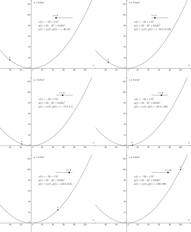
| − | + | [[Image:Cw df 1 notation 1.gif|thumb|left|400px|Fig 1: Example of curve parameterization]] | |
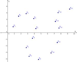
| + | [[Image:Cw df 1 notation 2 P.png|thumb|left|300px|Fig 2.a: The points in $X$-$Y$ plane]] | ||
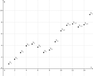
| + | [[Image:Cw df 1 notation 2 X.png|thumb|left|300px|Fig 2.b: X(t)]] | ||
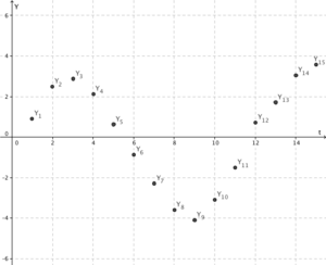
| + | [[Image:Cw df 1 notation 2 Y.png|thumb|left|300px|Fig 2.c: Y(t)]] | ||
| − | + | [[Image:Cw df 1 notation 4.png|thumb|left|200px|Fig 3: Straight line go through origin with slope 2]] | |
| − | + | In order to make the formulas for the same curve unanimous, we are going to introduce the concept of "arclength". First, we need to define the speed vector of the curve. For the curve C defined in above equation, its speed vector is defined as: | |
| − | + | ||
| − | + | ||
| − | + | ||
| − | + | ||
| − | + | ||
| − | + | ||
| − | + | ||
| − | + | ||
| − | + | ||
| − | + | ||
| − | + | ||
| − | + | ||
| − | + | ||
| − | + | ||
| − | + | ||
| − | + | ||
| − | + | ||
| − | + | ||
| − | + | ||
| − | + | ||
| − | + | ||
| − | First, we need to define the | + | |
<math> | <math> | ||
p^{\prime}(t)=\frac{d}{dt}p(t)=\left( \frac{d}{dt}x(t),\frac{d}{dt}y(t)\right). | p^{\prime}(t)=\frac{d}{dt}p(t)=\left( \frac{d}{dt}x(t),\frac{d}{dt}y(t)\right). | ||
| − | </math> | + | </math> |
| − | The | + | The speed, i.e. the magnitude of this speed vector, is: |
<math> | <math> | ||
| − | \| p^{\prime}(t)\| =\sqrt{\left( \frac{d}{dt}x(t)\right)^2+\left( \frac{d}{dt}y(t)\right)^2} | + | \| p^{\prime}(t)\| =\sqrt{\left( \frac{d}{dt}x(t)\right)^2+\left( \frac{d}{dt}y(t)\right)^2}. |
| − | </math> | + | </math> |
| − | + | For the same expressions of the straight line <span class="texhtml">''y'' = 2''x''</span> above, we know the corresponding speeds are: (a) <math>\|p^{\prime} (t)\| =\| (1,2)\|=\sqrt{5}</math>, (b) <math>\|p^{\prime} (t)\| =\| (2t,4t)\| =\sqrt{20} |t|</math>, and (c) <math>\| p^{\prime} (t)\| =\| \big( -\sin(t),-2\text{sin} (t) \big)\| =\sqrt{5} |\sin(t)|</math>. From these examples, we can see that the speed is not equal to the slope of the straight line. | |
| − | + | Now, we will uniquely parameterize the curve with respect to the "arclength" <span class="texhtml">''s''</span>, such that <math>\| \frac{d}{ds}p(s)\| =1</math>, <math>\forall s</math>, i.e. the unit speed parameterization. Hence, with any given parameter <span class="texhtml">''t''</span>, we can compute the derivative of <span class="texhtml">''p''(''t'')</span> with respect to the arclength <span class="texhtml">''s''</span> as following: <math> | |
| − | + | ||
| − | + | ||
| − | <math> | + | |
| − | + | ||
\frac{d}{ds}p(t)=\frac{p^{\prime}(t)}{\| p^{\prime}(t)\|}=\frac{\big( x^{\prime}(t),y^{\prime}(t)\big)}{\sqrt{\big( x^{\prime}(t)\big) ^2+\big( y^{\prime}(t)\big) ^2}}. | \frac{d}{ds}p(t)=\frac{p^{\prime}(t)}{\| p^{\prime}(t)\|}=\frac{\big( x^{\prime}(t),y^{\prime}(t)\big)}{\sqrt{\big( x^{\prime}(t)\big) ^2+\big( y^{\prime}(t)\big) ^2}}. | ||
| − | </math> | + | </math> |
| − | + | In other hand, we can also compute the same derivative with the chain rule: | |
<math> | <math> | ||
| − | + | \frac{d}{ds}p(t)=\frac{d}{dt}p(t)\cdot\frac{dt}{ds}=p^{\prime}(t)\cdot\frac{dt}{ds}. | |
| − | \frac{d}{ds}p(t)=\frac{d}{dt}p(t)\cdot\frac{dt}{ds}= p^{\prime}(t)\cdot\frac{dt}{ds}. | + | </math> |
| − | </math> | + | |
| + | Comparing above two equations, we can derive that: | ||
| − | |||
<math> | <math> | ||
\frac{dt}{ds}=\frac{1}{\sqrt{\big( x^{\prime}(t)\big) ^2+\big( y^{\prime}(t)\big) ^2}}\Rightarrow | \frac{dt}{ds}=\frac{1}{\sqrt{\big( x^{\prime}(t)\big) ^2+\big( y^{\prime}(t)\big) ^2}}\Rightarrow | ||
ds=\sqrt{\big( x^{\prime}(t)\big) ^2+\big( y^{\prime}(t)\big) ^2}dt=\|p^{\prime}(t)\| dt, | ds=\sqrt{\big( x^{\prime}(t)\big) ^2+\big( y^{\prime}(t)\big) ^2}dt=\|p^{\prime}(t)\| dt, | ||
| − | </math> | + | </math> |
| − | + | ||
| − | + | ||
| + | since <math>\| \frac{d}{ds}p(t)\| =1</math>. Then, we can easily compute the length of the curve <span class="texhtml">''p''(''t'')</span> from <span class="texhtml">''t'' = ''a''</span> to <span class="texhtml">''t'' = ''b''</span>: | ||
<math> | <math> | ||
| − | \int^{s(b)}_{s(a)}\| p^{\prime}(s)\| ds=\int^{s(b)}_{s(a)}1\cdot ds=\int^{b}_{a}\| p^{\prime}(t)\| dt=s(b)-s(a), | + | \int^{s(b)}_{s(a)}\|p^{\prime}(s)\| ds=\int^{s(b)}_{s(a)}1\cdot ds=\int^{b}_{a}\|p^{\prime}(t)\| dt=s(b)-s(a), |
| − | </math> | + | </math> |
| − | + | ||
| − | + | ||
| + | where <span class="texhtml">''s''(''t'')</span> is the parameter substitution function from <span class="texhtml">''t''</span> to <span class="texhtml">''s''</span>. For example, if <span class="texhtml">''p''(''s'')</span> is parameterized by arclength, the length of the curve from point <span class="texhtml">''p''(2)</span> to <span class="texhtml">''p''(17.5)</span> is <span class="texhtml">17.5 − 2 = 15.5</span>. | ||
---- | ---- | ||
[[Boutin_lectures_introduction_differential_geometry_Wu|Back to "Boutin lectures on Intro Differential geometry by Wu and Black"]] | [[Boutin_lectures_introduction_differential_geometry_Wu|Back to "Boutin lectures on Intro Differential geometry by Wu and Black"]] | ||
Revision as of 16:43, 14 May 2015
The Boutin Lectures on Introductory Differential Geometry
Slectures by Chyuan-Tyng "Roger" Wu and Will Black
2.1 blah
Notation
For a two-dimensional (2D) space $ \mathbb{R}^2 $, for example the X-Y plane, we can represent a smooth curve, C, in it as following:
$ C=\left\{ p(t):\big( x(t),y(t)\big) |t\in I\right\} $
, where I is some open interval of real number set $ \mathbb{R} $. The smooth curve indicates that the curve is differentiable everywhere (at least 3 times). Imaging we are drawing the this curve C in that plane with a pen, and then p(t) is the position of the pen at time t. Fig.1 and Figs.2 are two examples. However, the same curve C can have many different expressions. For example, the straight line that passes through the origin with slope 2, i.e. the straight in Fig.3, can be written as (a) $ \left\{\begin{array}{l}x(t)=t \\y(t)=2t\end{array}\right. $, (b) $ \left\{\begin{array}{l}x(t)=t^2 \\y(t)=2t^2\end{array}\right. $, or (c) $ \left\{\begin{array}{l}x(t)=\cos (t) \\y(t)=2\cos (t)\end{array}\right. $. Therefore, the spacing in time has nothing to do with the spacing in space.
In order to make the formulas for the same curve unanimous, we are going to introduce the concept of "arclength". First, we need to define the speed vector of the curve. For the curve C defined in above equation, its speed vector is defined as:
$ p^{\prime}(t)=\frac{d}{dt}p(t)=\left( \frac{d}{dt}x(t),\frac{d}{dt}y(t)\right). $
The speed, i.e. the magnitude of this speed vector, is:
$ \| p^{\prime}(t)\| =\sqrt{\left( \frac{d}{dt}x(t)\right)^2+\left( \frac{d}{dt}y(t)\right)^2}. $
For the same expressions of the straight line y = 2x above, we know the corresponding speeds are: (a) $ \|p^{\prime} (t)\| =\| (1,2)\|=\sqrt{5} $, (b) $ \|p^{\prime} (t)\| =\| (2t,4t)\| =\sqrt{20} |t| $, and (c) $ \| p^{\prime} (t)\| =\| \big( -\sin(t),-2\text{sin} (t) \big)\| =\sqrt{5} |\sin(t)| $. From these examples, we can see that the speed is not equal to the slope of the straight line.
Now, we will uniquely parameterize the curve with respect to the "arclength" s, such that $ \| \frac{d}{ds}p(s)\| =1 $, $ \forall s $, i.e. the unit speed parameterization. Hence, with any given parameter t, we can compute the derivative of p(t) with respect to the arclength s as following: $ \frac{d}{ds}p(t)=\frac{p^{\prime}(t)}{\| p^{\prime}(t)\|}=\frac{\big( x^{\prime}(t),y^{\prime}(t)\big)}{\sqrt{\big( x^{\prime}(t)\big) ^2+\big( y^{\prime}(t)\big) ^2}}. $
In other hand, we can also compute the same derivative with the chain rule:
$ \frac{d}{ds}p(t)=\frac{d}{dt}p(t)\cdot\frac{dt}{ds}=p^{\prime}(t)\cdot\frac{dt}{ds}. $
Comparing above two equations, we can derive that:
$ \frac{dt}{ds}=\frac{1}{\sqrt{\big( x^{\prime}(t)\big) ^2+\big( y^{\prime}(t)\big) ^2}}\Rightarrow ds=\sqrt{\big( x^{\prime}(t)\big) ^2+\big( y^{\prime}(t)\big) ^2}dt=\|p^{\prime}(t)\| dt, $
since $ \| \frac{d}{ds}p(t)\| =1 $. Then, we can easily compute the length of the curve p(t) from t = a to t = b: $ \int^{s(b)}_{s(a)}\|p^{\prime}(s)\| ds=\int^{s(b)}_{s(a)}1\cdot ds=\int^{b}_{a}\|p^{\prime}(t)\| dt=s(b)-s(a), $
where s(t) is the parameter substitution function from t to s. For example, if p(s) is parameterized by arclength, the length of the curve from point p(2) to p(17.5) is 17.5 − 2 = 15.5.
Back to "Boutin lectures on Intro Differential geometry by Wu and Black"


