| Line 3: | Line 3: | ||
Let us take a function <math>x(t)</math> | Let us take a function <math>x(t)</math> | ||
| − | [[Image:sampling_rate_conv.jpg | + | [[Image:sampling_rate_conv.jpg]] |
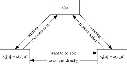
We wish to covert a signal sampled at <math>T_1</math> to one sampled at <math>T_2</math> without having to reconstruct the original <math>x(t)</math> and then resampling at a new rate. | We wish to covert a signal sampled at <math>T_1</math> to one sampled at <math>T_2</math> without having to reconstruct the original <math>x(t)</math> and then resampling at a new rate. | ||
| Line 72: | Line 72: | ||
[[Image:Xd_w.jpg|center]] | [[Image:Xd_w.jpg|center]] | ||
| + | |||
| + | We see that the scaled function is no longer periodic with period <math>2\pi</math>. | ||
| + | |||
| + | Now, consider frequency shifting the signal so that we have <math>\frac{1}{D}X_1(\frac{\omega-2\pi}{D})</math>. | ||
| + | |||
| + | [[Image:Xd2pi_w.jpg]] | ||
Revision as of 20:50, 22 September 2009
Sample Rate Conversion
Let us take a function $ x(t) $
We wish to covert a signal sampled at $ T_1 $ to one sampled at $ T_2 $ without having to reconstruct the original $ x(t) $ and then resampling at a new rate.
There are two cases here.
1. $ T_2 $ is a multiple of $ T_1 \to $ conversion can be accomplished by down-sampling
2. $ T_2 $ is a divider of $ T_1 \to $ conversion can be accomplished by up-sampling followed by LPF
Case 1 - $ T_2 $ is a multiple of $ T_1 $
We are trying to accomplish the following -
We know that
$ x_2[n] = x_1[Dn] \quad \mbox{where } D = \frac{T_2}{T_1} $
as this is the same as doing $ x_2[n] = x(T_2n) $
This, in Fourier Domain becomes
$ F(x_2[n]) = F(x_1[Dn]) $
$ X_2(\omega) = \sum_{n=-\infty}^{\infty} x_1[Dn] e^{-j \omega n} $
let $ m = Dn $
$ X_2(\omega) = \sum_{m=-\infty}^{\infty} x_1[m] e^{-j \omega \frac{m}{D}}\quad \mbox{where }m\mbox{ is a multiple of }D $
Now, we can introduce a function $ s_D[m] $ such that
$ s_D[m] = \begin{cases} 1, & \mbox{if }m\mbox{ multiple of }D\\ 0, & \mbox{else } \end{cases} $
The Fourier series of this function can be represented as
$ S_D[m] = \frac{1}{D} \sum_{k = 0}^{D-1} (e^{j \frac{2 \pi}{D} m})^k $
and therefore we get
$ X_2(\omega) = \sum_{m = -\infty}^{\infty} S_D[m] e^{-j \omega \frac{m}{D}} $
$ X_2(\omega) = \sum_{m = -\infty}^{\infty} \frac{1}{D}\sum_{k = 0}^{D-1} e^{j k \frac{2 \pi}{D} m} x_1[m] e^{-j \omega \frac{m}{D}} $
$ X_2(\omega) = \frac{1}{D} \sum_{k=0}^{D-1} \sum_{m=-\infty}^{\infty} x_1[m] e^{-j m (\frac{\omega - 2 \pi k}{D})} $
And since $ \sum_{m=-\infty}^{\infty} x_1[m] e^{-j m (\frac{\omega - 2 \pi k}{D})} = X_1(\frac{\omega - 2 \pi k}{D}) $
Therefore,
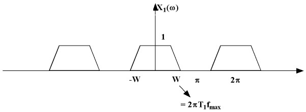
Let us assume the following plot for $ X_1(\omega) $. We will also assume that the Nyquist condition is satisfied, ie. $ f_{max} < \frac{1}{2T_1} $.
Now, on scaling we have the following plot for $ \frac{1}{D} X_1(\frac{\omega}{D}) $
We see that the scaled function is no longer periodic with period $ 2\pi $.
Now, consider frequency shifting the signal so that we have $ \frac{1}{D}X_1(\frac{\omega-2\pi}{D}) $.


