Contents
Logistic Models
I. Classic Logistic Models
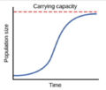
After realizing limitations of the exponential model, we may wonder: can we do better? We know that the resources are not unlimited. Therefore, at some point, the growth rate must slow down and eventually the population should reach the place where the environment cannot hold more. Based on the above description, it is reasonable to come up to a graph like this:
Caption1

Figure 1 An explanation of logistic growth model Adapted from Lumen Boundless Biology 2013
Mathematically, we have a model, which is called Logistic equation.
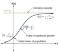
Caption2

Figure 2 An explanation about the growth rate changes over time Adapted from Lumen Boundless Biology For the moment, let’s just ignore the equation f(x) on the right. We’ll cover the mathematical part in the later section. Right now, we’re focusing on the actual meaning of this graph. Let’s check together whether this graph has all the features we discussed before.
By taking the tangent line of each pair of points along the x-axles, we find that the slope is indeed getting smaller and smaller. And when x is sufficiently large, the slope is close to 0. It means, the growth rate of population decreases in each period of years. And after a long time, the number of populations becomes stable. It makes sense intuitively. Please be aware that the decline of growth rate does not indicate the drop of population. On the contrary, the total population is still increasing as shown in the graph. For more advanced readers, the growth rate is represented by the derivative of the function. And the carrying capacity is the limit of the function when x approaches infinity.
The actual formula was first proposed by the Belgium mathematician Pierre-François Verhulst in 1835, who stated “The virtual increase of population is limited by the size and the fertility of the country. As a result, the population gets closer and closer to a steady state” in his Note on the law of population growth. (1838 as cited in Bacaër, 2011,)
Here N, K, r represent population, carrying capacity, and a growth rate parameter respectively. Noted the formula is given in the differentiation form.
This model assumes that the growth rate r is linear and it is decreasing in terms of N. In other words, r_a=F(N). For a more complete model, we will introduce r_m as the max growth rate. But it is beyond our text slope.
Interestingly, if N(t) is much smaller than K, this ordinary equation is approximately as our previous exponential model. Here comes another question. Can we write N(t) explicitly just like the exponential one?
The exciting answer is yes! But understanding how to get it requires some math background in an introductory level ordinary differential equation class. We strongly encourage interested readers take MA366 or MA 266 held by Purdue math department.
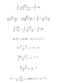
Let’s do some math!
Caption3

Figure 3 Merma, 2004 P80 The logistic equation Adapted from Northwestern University website
And we’ll see in later section that even the complicated logistic equation cannot predict the population accurately.
II.Theta Logistic model
We’ve already seen that even though logistic model does a better job on fitting the data of population than the exponential model does, the basic logistic model is still not the best model.
In order to fit better model and address the limitations set by the logistic model, Gilpin and Ayala(1973) presented a new version of the logistic model (as cited in Clark et al., 2010) called “theta logistic model”.
As a large population size continue to grow, individual growth rate should slow down which is not included in the classical model. The new theta-logistic model, however, take this into account. (Clark et al., 2010)
A new term θ is added to the classic logistic model. The linear density dependence held by the classical logistic model can be altered to become curvilinear. It is this new term θ that provides additional generality and flexibility to explain the impact by change of individual growth rate parameter r_a with respect to population density N. (Salisbury,2011)
How does θ work mathematically in this model? With the variation of θ, it can reflect relation between intraspecific competition and population density. In the classic logistic model, we have
![]() instead,
where r_m is the maximum growth rate which decrease linearly as N increases.
instead,
where r_m is the maximum growth rate which decrease linearly as N increases.
Now in the new theta logistic model, we have
 instead.
Notice that with θ=1, we have the basic logistic model; with θ=0, we have zero-growth.
instead.
Notice that with θ=1, we have the basic logistic model; with θ=0, we have zero-growth.
What happens when θ is taking other values then?
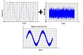
The following graph demonstrates four different cases with θ>1 or θ<1.

This graph shows a typical demonstration of how various values of θ alter the shape of the grows response curve with r_m=0.5 and K=100. As θ>1, when r>0, the growth response curve is concave down while as θ<1, the growth response curve is concave up.
And now we are ready to derive the new model!
After substituting our updated growth rate r_a into our original logistic equation, we obtain the theta-logistic growth model:
Caption1
Caption2

Notice that
Caption1
Caption2
That is when we set θ>1, the carrying capacity term has more weight(compares to previous model because the first term of the formula is smaller now), thus weakening the density-dependence for low values of N. And when we set θ<1, the density dependence is strengthened for low values of N, leading to slower population growth. These two different scenarios could be represented in the following graph:
Caption1
Caption2
caption((Phase line portrait of theta-logistic model, described by Eq. (2.28), for arbitrary values of θ = (0.5, 1, 3, 10) .(Salisbury,2011)))
Now, a question you may ask would be, is the model perfectly fit our census data of population? Unfortunately, the answer is still no.
In an research paper published in 2010, Francis et al. (2010) demonstrated that when they were fitting theta-logistic model with the most census data, it was not robust! With the time series they used, r was not a reliable estimation of the growth response rate. They concluded that more ecological clarification on the concept of carrying capacity is needed in order to develop further research study.
III.Logistic Model with Allee’s Effect
We talked about how the population grows and how carrying capacity works, but we have not seen what would happen if there is only a small population. The classical view of population dynamics expressed that the growth rate of a population will decrease at higher density and increase at lower density due to competition for limited resources. However, the Allee effect (derived from Warder Clyde Allee’s “Allee principle” introduced in the 1950s) described a situation in which when the density is low, the population growth rate also decreases because of, according to Alexander Salisbury’s Mathematical Models in Population Dynamics, “limited mate availability and impaired cooperative behaviors.” (2011, p.61) The following graph clearly shows the difference between the classical dynamics and Allee effect which has a positive density dependence, the positive correlation between population density and individual fitness (often measured as per capita population growth rate).

Adapted from Courchamp, Ludek, &Gascoigne, 2008.
According to Alexander, to begin incorporating the Allee effect into a normal logistic growth, we need to find the Allee threshold, above which the population will continue by ordinary logistic growth, and below which the population will decay (due to Allee effect) (2011). A simple mathematical example of an Allee effect from wikipedia (Salisbury, 2011, p.62) is given by the cubic growth model, $ \frac{dN}{dT}=rN(\frac{N}{T}-1)(1-\frac{N}{K}) $ where N = population size; r = intrinsic rate of increase; K = carrying capacity; T = Allee threshold; $ \frac{dN}{dT} $ = rate of increase of the population.

Dynamincs of the Allee effect. Adapted from “Mathematical Models in Population Dynamics,” by Alexander Salisbury, 2011.
This graph is an example of a strong Allee effect where the population has a negative growth rate for 0 < N < T and are eventually driven to extinction, and a positive growth rate for T < N < K (assuming 0 < T < K). In cases of a weak Allee effect, populations below the threshold are merely hampered in their rates of growth. The occurrences of Allee effect are more easily observed from small populations as populations above the threshold follow a logistic growth. Since human population has never dropped to such a low level, there is no research concerning about influence of Allee effect to human population, but Allee effect has been observed in many species, especially animals that hunt for prey or defend against predators as a group.
Indeed, predicting the population is a very difficult. It’s more than selecting several dots in the data and trying to come up with a fancy model from scratch. It also involves data collecting, analysis and some more advanced math like stochastic process as the real world has so many unexpected things happening that will influence the population size greatly. For curious readers, we have listed some references related to how population projections work in nowadays.
