m |
|||
| Line 1: | Line 1: | ||
| − | |||
| − | |||
LECTURE THEME : | LECTURE THEME : | ||
| Line 60: | Line 58: | ||
<math>P(w_1) \geq P(w_2)</math> decision is based on the prior<br> | <math>P(w_1) \geq P(w_2)</math> decision is based on the prior<br> | ||
| − | + | [[Category:Lecture Notes]] | |
| − | + | ||
| − | [ | + | |
| − | + | ||
| − | + | ||
| − | + | ||
Revision as of 22:13, 6 April 2008
LECTURE THEME :
Bayes classification
Topics:
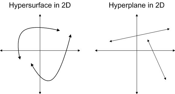
Clarification 1 - Difference between Hyperplane and Hypersurface: In simple terms, a hypersurface is any n-1 dimensional surface in n-dimensional space, while hyperplane is a flat hypersurface.
Clarification 2 - All classifiers are defined by hypersurfaces. - Consider a Nearest Neighbor classification problem: The classification of any query is decided by the label of its nearest neighbor. It may not be clear how this classifier can be defined by hypersurface. But we can define separating hypersurfaces which pass mid-way between points of different classes. In the extreme case, there can be a hypersurface for each data point enveloping all queries that will be classified with the label of that data point.
To find building blocks "g" or hypersurfaces of a classifier there are two approaches:
1)Supervised Learning: Somebody provides a category label in a training set. This collection of examples is used to infer the rules to categorize other examples. 2)Unsupervised Learning: Very related to "Clustering", or the "Discovery of groupings". These groupings become the unknown classes that we want to discover in the measurements. Nobody places labels in the training set. In many cases Supervised methods are applied within Unsupervised method to separate known classes within clusters.
- Follow Link to Zoubin Ghahramani's tutorial on Supervised, Reinforcement and Unsupervised Learning http://www.inf.ed.ac.uk/teaching/courses/pmr/docs/ul.pdf .
High Dimensional IssuesThe curse of dimensionality starts at d>17-23. There are no clusters or groupings of data points when d>17. In practice each point turns to be a cluster on its own and as a result this explodes into a high dimensional feature vectors which are impossible to handle in computation.
Bayes rule
Bayes rule addresses the predefined classes classification problem. Given value of X for an object, assign one of the k classes to the object
Bayes rule for discrete feature vector Bayes rule is to do the following: Given x=x, choose the most likely class $ E{\lbrace}w_1,...,w_k{\rbrace} $
$ w: E{\lbrace}w_1,...,w_k{\rbrace} $ ie. choose $ w_i $ such that the $ P(w_i|x) \geq P(w_j|x), {\forall}j $
$ posterior = \frac{(likelihood)(prior)}{(evidence)} $
$ posterior = P(w_i|x)= \frac{p(x|w_i)P(w_i)}{P(x)} $
Bayes rule: choose the class $ w_i $ that maximizes the $ p(x|w_i)P(w_i) $
Example: Given 2 class decision problems $ w_1 = $ women & $ w_2 $= men, $ L = hair length $ choose $ w_1 $, if $ P(w_1|L) \geq P(w_2|L) $ else choose $ w_2 $ or
choose $ w_1 $ if $ p(L|w_1)P(w_1)>p(L|w_2)P(w_2) $
else choose $ w_2 $
Minimum probability of error is the error made when $ w = w_2 $ and decided $ w_1 $
Special cases
If $ P(w_1) = P(w_2) $
$ p(x|w_1)P(w_1) \geq p(x|w_2)P(w_2), {\forall j} $
$ p(x|w_1) \geq p(x|w_2) $ decision is based on the likelihood
-If $ p(x|w_1)=p(x|w_2) $
$ p(x|w_1)P(w_1) \geq p(x|w_2)P(w_2), {\forall j} $
$ P(w_1) \geq P(w_2) $ decision is based on the prior


