The perceptron algorithm maps an input to a single binary output value. For a proof of the Perceptron convergence theorem, see [PerceptronConvergenceTheorem]
First introduced in [Lecture 9]. The gradient descent algorithm used is discussed in [Lecture 10].
Contents
Gradient Descent
Main article: Gradient Descent_OldKiwi
Consider the cost function $ J_p(\vec{c}) = \sum -\vec{c}y_i $, where $ y_i $ is the misclassified data.
We use the gradient descent procedure to minimize $ J_p(\vec{c}) $.
Compute $ \nabla J_p(\vec{c}) = ... = - \sum y_i $.
Follow basic gradient descent procedure:
- Initial guess $ \vec{c_1} $
- Then, update $ \vec{c_2} = \vec{c_1} - \eta(1) \nabla J_p(\vec{c}) $, where $ \eta(1) $ is the step size
- Iterate $ \vec{c_{k+1}} = \vec{c_{k}} - \eta(k) \nabla J_p(\vec{c}) $until it "converges"
( e.g when $ \eta(k) \nabla J_p(\vec{c}) $< threshold )
Gradient Descent in the Perceptron Algorithm
- Theorem: If samples are linearly separable, then the "batch [perceptron]" iterative algorithm. The proof of this theorem, PerceptronConvergenceTheorem, is due to Novikoff (1962).
$ \vec{c_{k+1}} = \vec{c_k} + cst \sum y_i $, where $ y_i $ is the misclassified data, terminates after a finite number of steps.
But, in practice, we do not have linear separable data. So instead, we use the Least Squares Procedure.
We want $ \vec{c} \cdot y_i > 0 $, for all samples $ y_i $. This is a linear inequality problem which is usually hard to solve. Therefore, we need to convert this problem into a linear equality problem.
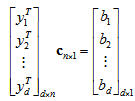
We choose $ b_i $ > 0 and solve $ \vec{c} \cdot y_i = b_i $, for all i
The matrix equation has the following form:
This can also be written as $ \vec{Y} \cdot \vec{c} = \vec{b} $
If d=n, and $ \vec{y_1} $,..., $ \vec{y_d} $ are "generic" ( i.e. determinant of $ \vec{Y} $ is not 0), then we "can" solve by matrix inversion.
If d > n, over-constrained system (there is no solution in the generic case). This is the case where there is more data than you need, and the information is contradictory. In this case, we seek to minimize $ || Y \vec{c} - \vec{b} ||_{L_2} $. The solution is given by $ \vec{c} = (Y^{\top}Y)^{-1}Y^{\top}b $, if $ |Y^{\top}y| \ne 0 $.
If $ |Y^{\top}y| = 0 $, $ \vec{c} = lim (Y^{\top}Y + \epsilon1)^{-1}Y^{\top}b $ always exists!
Fischer's Linear Discriminant
Main article: Fisher Linear Discriminant_OldKiwi
Fischer's Linear Discriminant solves a dual problem: Traditionally, we have defined a separating hyperplane. Fischer's linear discriminant defines a projection which reduced the data to a single dimension.
Fischer's Linear Discriminant optimizes the between class-spread.


