The perceptron algorithm maps an input to a single binary output value. For a proof of the Perceptron convergence theorem, see [PerceptronConvergenceTheorem]
First introduced in [Lecture 9]. The gradient descent algorithm used is discussed in [Lecture 10].
Contents
Gradient Descent
Main article: Gradient Descent_OldKiwi
Consider the cost function $ J_p(\vec{c}) = \sum -\vec{c}y_i $, where $ y_i $ is the misclassified data.
We use the gradient descent procedure to minimize $ J_p(\vec{c}) $.
Compute $ \nabla J_p(\vec{c}) = ... = - \sum y_i $.
Follow basic gradient descent procedure:
- Initial guess $ \vec{c_1} $
- Then, update $ \vec{c_2} = \vec{c_1} - \eta(1) \nabla J_p(\vec{c}) $, where $ \eta(1) $ is the step size
- Iterate $ \vec{c_{k+1}} = \vec{c_{k}} - \eta(k) \nabla J_p(\vec{c}) $until it "converges"
( e.g when $ \eta(k) \nabla J_p(\vec{c}) $< threshold )
Gradient Descent in the Perceptron Algorithm
- Theorem: If samples are linearly separable, then the "batch [perceptron]" iterative algorithm. The proof of this theorem, PerceptronConvergenceTheorem, is due to Novikoff (1962).
$ \vec{c_{k+1}} = \vec{c_k} + cst \sum y_i $, where $ y_i $ is the misclassified data, terminates after a finite number of steps.
But, in practice, we do not have linear separable data. So instead, we use the Least Squares Procedure.
We want $ \vec{c} \cdot y_i > 0 $, for all samples $ y_i $. This is a linear inequality problem which is usually hard to solve. Therefore, we need to convert this problem into a linear equality problem.
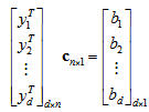
We choose $ b_i $ > 0 and solve $ \vec{c} \cdot y_i = b_i $, for all i
The matrix equation has the following form:
This can also be written as $ \vec{Y} \cdot \vec{c} = \vec{b} $
If d=n, and $ \vec{y_1} $,..., $ \vec{y_d} $ are "generic" ( i.e. determinant of $ \vec{Y} $ is not 0), then we "can" solve by matrix inversion.
If d > n, over-constrained system (there is no solution in the generic case). This is the case where there is more data than you need, and the information is contradictory. In this case, we seek to minimize $ || Y \vec{c} - \vec{b} ||_{L_2} $. The solution is given by $ \vec{c} = (Y^{\top}Y)^{-1}Y^{\top}b $, if $ |Y^{\top}y| \ne 0 $.
If $ |Y^{\top}y| = 0 $, $ \vec{c} = lim (Y^{\top}Y + \epsilon1)^{-1}Y^{\top}b $ always exists!
Fischer's Linear Discriminant
Main article: Fisher Linear Discriminant_OldKiwi
Introduction
==
Fischer's Linear Discriminant solves a dual problem: Traditionally, we have defined a separating hyperplane. Fischer's linear discriminant defines a projection which reduced the data to a single dimension.
Fischer's Linear Discriminant optimizes the between class-spread.
Fisher's linear discriminant is a classification method that projects high-dimensional data onto a line and performs classification in this one-dimensional space. The projection maximizes the distance between the means of the two classes while minimizing the variance within each class. See [Lecture 10] for detailed explanation.
Finding the separating hyperplane and finding the projection direction are dual problems
=======================================
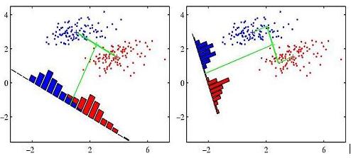
Fisher's Linear Discriminant relies on dimension reduction. If we want to project D-dimensional data down to one dimension we can use $ y=\omega^T \vec{x} $ . After that, by determining a threshold $ \omega_0 $, we can select class 1 if $ y>\omega_0 $ and class 2 if $ y<\omega_0> $.
However, dimension reduction can cause considerable amount of information loss leading not being able to separate the data in reduced dimension, while the data is separable in D dimension. Fisher's Linear Discriminant method uses that idea by adjusting the weight vector $ \omega $ for projection to minimize the amount of overlapping data in reduced dimension. Here are some figures from C. M. Bishop's book to understand the idea completely.
- Context:** Classical [Discriminant Analysis] Problem
Given data $ y_1,\cdots, y_d \in \mathbb{R}^n $, from 2 classes. When n is big, it may be difficult to separate classes, because of computational issues.
In this case we try to find a projection $ \pi: R^n \rightarrow R^k, k <n $ s.t . $ \pi(y_1), \cdots, \pi(y_d) $ can be separated.
Derivation of Fisher's Linear Discriminant
================
Main article: [Derivation of Fisher's Linear Discriminant]
References
=
"`Two variations on Fisher's linear discriminant for pattern recognition <http://ieeexplore.ieee.org/Xplore/login.jsp?url=/iel5/34/21179/00982904.pdf>`_" is a nice journal article. The paper provides two fast and simple techniques for improving on the classification performance provided by Fisher's linear discriminant for two classes. See the following link for the detailed information: `Two variations on Fisher's linear discriminant for pattern recognition <http://ieeexplore.ieee.org/Xplore/login.jsp?url=/iel5/34/21179/00982904.pdf>`_.


