| Line 29: | Line 29: | ||
:<math>x_r(t) = \sum_{k=-\infty}^{\infty} x(kT) \cdot sinc(t/T) * \delta(t - kT)</math> | :<math>x_r(t) = \sum_{k=-\infty}^{\infty} x(kT) \cdot sinc(t/T) * \delta(t - kT)</math> | ||
| − | When | + | When convolving a function with a shifted delta, the result is the function shifted |
:<math>x_r(t) = \sum_{k=-\infty}^{\infty} x(kT) \cdot sinc(\frac{t-kT}{T})</math> | :<math>x_r(t) = \sum_{k=-\infty}^{\infty} x(kT) \cdot sinc(\frac{t-kT}{T})</math> | ||
Latest revision as of 19:51, 22 September 2009
HW3_Signal Reconstruction_Interpolation (Band-limited)
After having creating a sampled version of the original function, $ X_{s} $, it needs to be reconstructed into the original function $ x(t) $. To do this, the Whittaker-Shannon interpolation formula is utilized.
The sampling theorem says that given a function that meets two requirements:
- 1) It is band-limited. This means that the Fourier transform of the original signal, also known as the spectrum, is 0 for |f| > B, where B is the bandwidth.
- 2) It is sampled at the Nyquist frequency, $ f_s > 2B $
it can be exactly reconstructed from its samples. If it does not meet these two requirements, aliasing occurs.
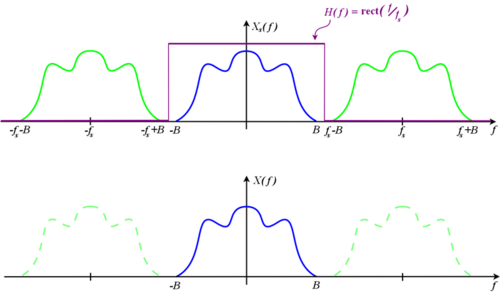
To recover the signal, the sampled function is simply multiplied by a low-pass filter with height equal to the sampling period T, $ {H_r}(f) $, to isolate the original signal.
$ {X_r}(f) = {H_r}(f){X_s}(f) $
Mathematical Process for finding $ {X_r}(f) $:
$ {X_r}(f) = {H_r}(f) \cdot {X_s}(f) $ where $ {H_r}(f) = T {rect}(Tf) $
Convert to the time domain. $ X_s(f) $ in the time domain is the sum of a train of deltas at every period of sampling, T
- $ x_r(t) = h_r(t) * x_s(t) = sinc(t/T) * \sum_{k=-\infty}^{\infty} x(kT)\cdot \delta(t - kT) $
Properties of convolution allow
- $ x_r(t) = \sum_{k=-\infty}^{\infty} x(kT) \cdot sinc(t/T) * \delta(t - kT) $
When convolving a function with a shifted delta, the result is the function shifted
- $ x_r(t) = \sum_{k=-\infty}^{\infty} x(kT) \cdot sinc(\frac{t-kT}{T}) $
It should be noted that while this may work in the theoretical, it is impossible to make a low-pass filter with an infinite cut-off slope. It is for this reason oversampling is used when reconstructing the signal. Oversampling inserts zeros after every sample according to the oversampling factor D. As an example, if D=4, the system would insert three samples of value zero in between each of the old samples. The sampled output spectrum will still repeat periodically, just with 4 times the period. Additionally an analog filter will have to be used to filter the sampled output.
Reference: http://www.silcom.com/~aludwig/Signal_processing/Signal_processing.htm#Resolution_and_bandwidth


