(New page: == Part B: Find the Bug == The original Matlab code: <br> F0 =13; <br> T0 =1/F0; <br> Ts = 0.07;<br> t = 0:Ts:13*T0;<br> x = real(exp(j*(2*pi*F0*t-pi/2)));<br> plot(t,x)<br> This code ...) |
(→Part B: Find the Bug) |
||
| (One intermediate revision by the same user not shown) | |||
| Line 15: | Line 15: | ||
F0 =13; <br> | F0 =13; <br> | ||
T0 =1/F0; <br> | T0 =1/F0; <br> | ||
| − | Ts = 0. | + | Ts = 0.01*T0;<br> |
t = 0:Ts:13*T0;<br> | t = 0:Ts:13*T0;<br> | ||
x = real(exp(j*(2*pi*F0*t-pi/2)));<br> | x = real(exp(j*(2*pi*F0*t-pi/2)));<br> | ||
plot(t,x)<br> | plot(t,x)<br> | ||
| + | |||
| + | [[Image:Untitled5_ECE301Fall2008mboutin.jpg]] | ||
Latest revision as of 15:21, 10 September 2008
Part B: Find the Bug
The original Matlab code:
F0 =13;
T0 =1/F0;
Ts = 0.07;
t = 0:Ts:13*T0;
x = real(exp(j*(2*pi*F0*t-pi/2)));
plot(t,x)
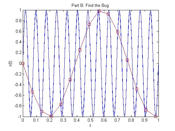
This code produces an accurate plot of the real part of the signal it is attempting to plot. However, because the sampling frequency is so large, the plotted points make the signal look as if it is not periodic. In order to correct this mistake, the variable Ts needs to be much smaller.
New Matlab code:
F0 =13;
T0 =1/F0;
Ts = 0.01*T0;
t = 0:Ts:13*T0;
x = real(exp(j*(2*pi*F0*t-pi/2)));
plot(t,x)


